Sequent calculus
m (markup fixes) |
(→Equivalence: Link to List of equivalences) |
||
| (20 intermediate revisions by 3 users not shown) | |||
| Line 1: | Line 1: | ||
This article presents the language and sequent calculus of second-order |
This article presents the language and sequent calculus of second-order |
||
| − | propositional linear logic and the basic properties of this sequent calculus. |
+ | linear logic and the basic properties of this sequent calculus. |
| − | + | The core of the article uses the two-sided system with negation as a proper |
|
| − | + | connective; the [[#One-sided sequent calculus|one-sided system]], often used |
|
| + | as the definition of linear logic, is presented at the end of the page. |
||
== Formulas == |
== Formulas == |
||
| − | Formulas are built on a set of atoms, written <math>\alpha,\beta,\ldots</math>, that can |
+ | Atomic formulas, written <math>\alpha,\beta,\gamma</math>, are predicates of |
| − | be either propositional variables <math>X,Y,Z\ldots</math> or atomic formulas |
+ | the form <math>p(t_1,\ldots,t_n)</math>, where the <math>t_i</math> are terms |
| − | <math>X(t_1,\ldots,t_n)</math>, where the <math>t_i</math> are terms from some first-order language. |
+ | from some first-order language. |
| − | Formulas, represented by capital letters <math>A</math>, <math>B</math>, <math>C</math>, are built using the |
+ | The predicate symbol <math>p</math> may be either a predicate constant or a |
| − | following connectives: |
+ | second-order variable. |
| + | By convention we will write first-order variables as <math>x,y,z</math>, |
||
| + | second-order variables as <math>X,Y,Z</math>, and <math>\xi</math> for a |
||
| + | variable of arbitrary order (see [[Notations]]). |
||
| − | <math> |
+ | Formulas, represented by capital letters <math>A</math>, <math>B</math>, |
| − | \begin{array}{clcll} |
+ | <math>C</math>, are built using the following connectives: |
| − | \alpha & \text{atom} & |
||
| − | \alpha\orth & \text{negated atom} & \text{atoms} \\ |
||
| − | A \tens B & \text{tensor} & |
||
| − | A \parr B & \text{par} & \text{multiplicatives} \\ |
||
| − | \one & \text{one} & |
||
| − | \bot & \text{bottom} & \text{multiplicative units} \\ |
||
| − | A \plus B & \text{plus} & |
||
| − | A \with B & \text{with} & \text{additives} \\ |
||
| − | \zero & \text{zero} & |
||
| − | \top & \text{top} & \text{additive units} \\ |
||
| − | \oc A & \text{of course} & |
||
| − | \wn A & \text{why not} & \text{exponentials} \\ |
||
| − | \exists x.A & \text{there exists} & |
||
| − | \forall x.A & \text{for all} & \text{quantifiers} |
||
| − | \end{array} |
||
| − | </math> |
||
| − | Each line corresponds to a particular class of connectives, and each class |
+ | {| style="border-spacing: 2em 0" |
| − | consists in a pair of connectives. |
||
| − | Those in the left column are called positive and those in the right column are |
||
| − | called negative. |
||
| − | The ''tensor'' and ''with'' are conjunctions while ''par'' and |
||
| − | ''plus'' are disjunctions. |
||
| − | The exponential connectives are called ''modalities'', and traditionally |
||
| − | read ''of course <math>A</math>'' for <math>\oc A</math> and ''why not <math>A</math>'' for <math>\wn A</math>. |
||
| − | Quantifiers may apply to first- or second-order variables. |
||
| − | |||
| − | |||
| − | Given a formula <math>A</math>, its linear negation, also called ''orthogonal'' and |
||
| − | written <math>A\orth</math>, is obtained by exchanging each positive connective with the |
||
| − | negative one of the same class and vice versa, in a way analogous to de Morgan |
||
| − | laws in classical logic. |
||
| − | Formally, the definition of linear negation is |
||
| − | |||
| − | {| |
||
|- |
|- |
||
| − | |align="right"|   <math> |
+ | | <math>\alpha</math> |
| − | ( \alpha )\orth </math> |
+ | | atom |
| − | | <math>:= \alpha\orth </math> |
+ | | <math>A\orth</math> |
| − | |align="right"|   <math> |
+ | | negation |
| − | ( \alpha\orth )\orth </math> |
||
| − | | <math>:= \alpha </math> |
||
|- |
|- |
||
| − | |align="right"|   <math> |
+ | | <math>A \tens B</math> |
| − | ( A \tens B )\orth </math> |
+ | | tensor |
| − | | <math>:= A\orth \parr B\orth </math> |
+ | | <math>A \parr B</math> |
| − | |align="right"|   <math> |
+ | | par |
| − | ( A \parr B )\orth </math> |
+ | | multiplicatives |
| − | | <math>:= A\orth \tens B\orth </math> |
||
|- |
|- |
||
| − | |align="right"|   <math> |
+ | | <math>\one</math> |
| − | \one\orth </math> |
+ | | one |
| − | | <math>:= \bot </math> |
+ | | <math>\bot</math> |
| − | |align="right"|   <math> |
+ | | bottom |
| − | \bot\orth </math> |
+ | | multiplicative units |
| − | | <math>:= \one </math> |
||
|- |
|- |
||
| − | |align="right"|   <math> |
+ | | <math>A \plus B</math> |
| − | ( A \plus B )\orth </math> |
+ | | plus |
| − | | <math>:= A\orth \with B\orth </math> |
+ | | <math>A \with B</math> |
| − | |align="right"|   <math> |
+ | | with |
| − | ( A \with B )\orth </math> |
+ | | additives |
| − | | <math>:= A\orth \plus B\orth </math> |
||
|- |
|- |
||
| − | |align="right"|   <math> |
+ | | <math>\zero</math> |
| − | \zero\orth </math> |
+ | | zero |
| − | | <math>:= \top </math> |
+ | | <math>\top</math> |
| − | |align="right"|   <math> |
+ | | top |
| − | \top\orth </math> |
+ | | additive units |
| − | | <math>:= \zero </math> |
||
|- |
|- |
||
| − | |align="right"|   <math> |
+ | | <math>\oc A</math> |
| − | ( \oc A )\orth </math> |
+ | | of course |
| − | | <math>:= \wn ( A\orth ) </math> |
+ | | <math>\wn A</math> |
| − | |align="right"|   <math> |
+ | | why not |
| − | ( \wn A )\orth </math> |
+ | | exponentials |
| − | | <math>:= \oc ( A\orth ) </math> |
||
|- |
|- |
||
| − | |align="right"|   <math> |
+ | | <math>\exists \xi.A</math> |
| − | ( \exists X.A )\orth </math> |
+ | | there exists |
| − | | <math>:= \forall X.( A\orth ) </math> |
+ | | <math>\forall \xi.A</math> |
| − | |align="right"|   <math> |
+ | | for all |
| − | ( \forall X.A )\orth </math> |
+ | | quantifiers |
| − | | <math>:= \exists X.( A\orth ) |
||
| − | </math> |
||
|} |
|} |
||
| − | Note that this operation is defined syntactically, hence negation is not a |
+ | Each line (except the first one) corresponds to a particular class of |
| − | connective, the only place in formulas where the symbol <math>(\cdot)\orth</math> occurs |
+ | connectives, and each class consists in a pair of connectives. |
| − | is for negated atoms <math>\alpha\orth</math>. |
+ | Those in the left column are called [[positive formula|positive]] and those in |
| − | Note also that, by construction, negation is involutive: for any formula <math>A</math>, |
+ | the right column are called [[negative formula|negative]]. |
| − | it holds that <math>A\biorth=A</math>. |
+ | The ''tensor'' and ''with'' connectives are conjunctions while ''par'' and |
| + | ''plus'' are disjunctions. |
||
| + | The exponential connectives are called ''modalities'', and traditionally read |
||
| + | ''of course <math>A</math>'' for <math>\oc A</math> and ''why not |
||
| + | <math>A</math>'' for <math>\wn A</math>. |
||
| + | Quantifiers may apply to first- or second-order variables. |
||
There is no connective for implication in the syntax of standard linear logic. |
There is no connective for implication in the syntax of standard linear logic. |
||
Instead, a ''linear implication'' is defined similarly to the decomposition |
Instead, a ''linear implication'' is defined similarly to the decomposition |
||
| − | <math>A\imp B=\neg A\vee B</math> in classical logic: |
+ | <math>A\imp B=\neg A\vee B</math> in classical logic, as |
| + | <math>A\limp B:=A\orth\parr B</math>. |
||
| − | <math> |
+ | Free and bound variables and first-order substitution are defined in the |
| − | A \limp B := A\orth \parr B |
+ | standard way. |
| − | </math> |
||
| − | |||
| − | |||
| − | Free and bound variables are defined in the standard way, as well as |
||
| − | substitution. |
||
Formulas are always considered up to renaming of bound names. |
Formulas are always considered up to renaming of bound names. |
||
| − | If <math>A</math> and <math>B</math> are formulas and <math>X</math> is a propositional variable, the formula |
+ | If <math>A</math> is a formula, <math>X</math> is a second-order variable and |
| − | <math>A[B/X]</math> is <math>A</math> where all atoms <math>X</math> are replaced (without capture) by <math>B</math> and |
+ | <math>B[x_1,\ldots,x_n]</math> is a formula with variables <math>x_i</math>, |
| − | all atoms <math>X\orth</math> are replaced by the formula <math>B\orth</math>. |
+ | then the formula <math>A[B/X]</math> is <math>A</math> where every atom |
| − | + | <math>X(t_1,\ldots,t_n)</math> is replaced by <math>B[t_1,\ldots,t_n]</math>. |
|
== Sequents and proofs == |
== Sequents and proofs == |
||
| − | A sequent is an expression <math>\vdash\Gamma</math> where <math>\Gamma</math> is a finite multiset |
+ | A sequent is an expression <math>\Gamma\vdash\Delta</math> where |
| − | of formulas. |
+ | <math>\Gamma</math> and <math>\Delta</math> are finite multisets of formulas. |
| − | For a multiset <math>\Gamma=A_1,\ldots,A_n</math>, the notation <math>\wn\Gamma</math> represents |
+ | For a multiset <math>\Gamma=A_1,\ldots,A_n</math>, the notation |
| − | the multiset <math>\wn A_1,\ldots,\wn A_n</math>. |
+ | <math>\wn\Gamma</math> represents the multiset |
| + | <math>\wn A_1,\ldots,\wn A_n</math>. |
||
Proofs are labelled trees of sequents, built using the following inference |
Proofs are labelled trees of sequents, built using the following inference |
||
rules: |
rules: |
||
| − | + | * Identity group: <math> |
|
| − | + | \LabelRule{\rulename{axiom}} |
|
| − | * Identity group:<br><math> |
+ | \NulRule{ A \vdash A } |
| − | \LabelRule{axiom} |
||
| − | \NulRule{ \vdash A, A\orth } |
||
\DisplayProof |
\DisplayProof |
||
| − | \qquad |
+ | </math>   <math> |
| − | \AxRule{ \vdash \Gamma, A } |
+ | \AxRule{ \Gamma \vdash A, \Delta } |
| − | \AxRule{ \vdash \Delta, A\orth } |
+ | \AxRule{ \Gamma', A \vdash \Delta' } |
| − | \LabelRule{cut} |
+ | \LabelRule{\rulename{cut}} |
| − | \BinRule{ \vdash \Gamma, \Delta } |
+ | \BinRule{ \Gamma, \Gamma' \vdash \Delta, \Delta' } |
\DisplayProof |
\DisplayProof |
||
</math> |
</math> |
||
| − | + | * Negation: <math> |
|
| − | + | \AxRule{ \Gamma \vdash A, \Delta } |
|
| − | * Multiplicative group:<br><math> |
+ | \UnaRule{ \Gamma, A\orth \vdash \Delta } |
| − | \AxRule{ \vdash \Gamma, A } |
+ | \LabelRule{n_L} |
| − | \AxRule{ \vdash \Delta, B } |
||
| − | \LabelRule{ \tens } |
||
| − | \BinRule{ \vdash \Gamma, \Delta, A \tens B } |
||
\DisplayProof |
\DisplayProof |
||
| − | \qquad |
+ | </math>   <math> |
| − | \AxRule{ \vdash \Gamma, A, B } |
+ | \AxRule{ \Gamma, A \vdash \Delta } |
| − | \LabelRule{ \parr } |
+ | \UnaRule{ \Gamma \vdash A\orth, \Delta } |
| − | \UnaRule{ \vdash \Gamma, A \parr B } |
+ | \LabelRule{n_R} |
\DisplayProof |
\DisplayProof |
||
| − | \qquad |
+ | </math> |
| − | \LabelRule{ \one } |
+ | * Multiplicative group: |
| + | ** tensor: <math> |
||
| + | \AxRule{ \Gamma, A, B \vdash \Delta } |
||
| + | \LabelRule{ \tens_L } |
||
| + | \UnaRule{ \Gamma, A \tens B \vdash \Delta } |
||
| + | \DisplayProof |
||
| + | </math>   <math> |
||
| + | \AxRule{ \Gamma \vdash A, \Delta } |
||
| + | \AxRule{ \Gamma' \vdash B, \Delta' } |
||
| + | \LabelRule{ \tens_R } |
||
| + | \BinRule{ \Gamma, \Gamma' \vdash A \tens B, \Delta, \Delta' } |
||
| + | \DisplayProof |
||
| + | </math> |
||
| + | ** par: <math> |
||
| + | \AxRule{ \Gamma, A \vdash \Delta } |
||
| + | \AxRule{ \Gamma', B \vdash \Delta' } |
||
| + | \LabelRule{ \parr_L } |
||
| + | \BinRule{ \Gamma, \Gamma', A \parr B \vdash \Delta, \Delta' } |
||
| + | \DisplayProof |
||
| + | </math>   <math> |
||
| + | \AxRule{ \Gamma \vdash A, B, \Delta } |
||
| + | \LabelRule{ \parr_R } |
||
| + | \UnaRule{ \Gamma \vdash A \parr B, \Delta } |
||
| + | \DisplayProof |
||
| + | </math> |
||
| + | ** one: <math> |
||
| + | \AxRule{ \Gamma \vdash \Delta } |
||
| + | \LabelRule{ \one_L } |
||
| + | \UnaRule{ \Gamma, \one \vdash \Delta } |
||
| + | \DisplayProof |
||
| + | </math>   <math> |
||
| + | \LabelRule{ \one_R } |
||
\NulRule{ \vdash \one } |
\NulRule{ \vdash \one } |
||
\DisplayProof |
\DisplayProof |
||
| − | \qquad |
+ | </math> |
| − | \AxRule{ \vdash \Gamma } |
+ | ** bottom: <math> |
| − | \LabelRule{ \bot } |
+ | \LabelRule{ \bot_L } |
| − | \UnaRule{ \vdash \Gamma, \bot } |
+ | \NulRule{ \bot \vdash } |
| + | \DisplayProof |
||
| + | </math>   <math> |
||
| + | \AxRule{ \Gamma \vdash \Delta } |
||
| + | \LabelRule{ \bot_R } |
||
| + | \UnaRule{ \Gamma \vdash \bot, \Delta } |
||
\DisplayProof |
\DisplayProof |
||
</math> |
</math> |
||
| − | + | * Additive group: |
|
| − | + | ** plus: <math> |
|
| − | * Additive group:<br><math> |
+ | \AxRule{ \Gamma, A \vdash \Delta } |
| − | \AxRule{ \vdash \Gamma, A } |
+ | \AxRule{ \Gamma, B \vdash \Delta } |
| − | \LabelRule{ \plus_1 } |
+ | \LabelRule{ \plus_L } |
| − | \UnaRule{ \vdash \Gamma, A \plus B } |
+ | \BinRule{ \Gamma, A \plus B \vdash \Delta } |
\DisplayProof |
\DisplayProof |
||
| − | \qquad |
+ | </math>   <math> |
| − | \AxRule{ \vdash \Gamma, B } |
+ | \AxRule{ \Gamma \vdash A, \Delta } |
| − | \LabelRule{ \plus_2 } |
+ | \LabelRule{ \plus_{R1} } |
| − | \UnaRule{ \vdash \Gamma, A \plus B } |
+ | \UnaRule{ \Gamma \vdash A \plus B, \Delta } |
\DisplayProof |
\DisplayProof |
||
| − | \qquad |
+ | </math>   <math> |
| − | \AxRule{ \vdash \Gamma, A } |
+ | \AxRule{ \Gamma \vdash B, \Delta } |
| − | \AxRule{ \vdash \Gamma, B } |
+ | \LabelRule{ \plus_{R2} } |
| − | \LabelRule{ \with } |
+ | \UnaRule{ \Gamma \vdash A \plus B, \Delta } |
| − | \BinRule{ \vdash, \Gamma, A \with B } |
||
\DisplayProof |
\DisplayProof |
||
| − | \qquad |
+ | </math> |
| − | \LabelRule{ \top } |
+ | ** with: <math> |
| − | \NulRule{ \vdash \Gamma, \top } |
+ | \AxRule{ \Gamma, A \vdash \Delta } |
| + | \LabelRule{ \with_{L1} } |
||
| + | \UnaRule{ \Gamma, A \with B \vdash \Delta } |
||
| + | \DisplayProof |
||
| + | </math>   <math> |
||
| + | \AxRule{ \Gamma, B \vdash \Delta } |
||
| + | \LabelRule{ \with_{L2} } |
||
| + | \UnaRule{ \Gamma, A \with B \vdash \Delta } |
||
| + | \DisplayProof |
||
| + | </math>   <math> |
||
| + | \AxRule{ \Gamma \vdash A, \Delta } |
||
| + | \AxRule{ \Gamma \vdash B, \Delta } |
||
| + | \LabelRule{ \with_R } |
||
| + | \BinRule{ \Gamma \vdash A \with B, \Delta } |
||
\DisplayProof |
\DisplayProof |
||
</math> |
</math> |
||
| − | + | ** zero: <math> |
|
| − | + | \LabelRule{ \zero_L } |
|
| − | * Exponential group:<br><math> |
+ | \NulRule{ \Gamma, \zero \vdash \Delta } |
| − | \AxRule{ \vdash \Gamma, A } |
||
| − | \LabelRule{ d } |
||
| − | \UnaRule{ \vdash \Gamma, \wn A } |
||
\DisplayProof |
\DisplayProof |
||
| − | \qquad |
+ | </math> |
| − | \AxRule{ \vdash \Gamma } |
+ | ** top: <math> |
| − | \LabelRule{ w } |
+ | \LabelRule{ \top_R } |
| − | \UnaRule{ \vdash \Gamma, \wn A } |
+ | \NulRule{ \Gamma \vdash \top, \Delta } |
\DisplayProof |
\DisplayProof |
||
| − | \qquad |
+ | </math> |
| − | \AxRule{ \vdash \Gamma, \wn A, \wn A } |
+ | * Exponential group: |
| − | \LabelRule{ c } |
+ | ** of course: <math> |
| − | \UnaRule{ \vdash \Gamma, \wn A } |
+ | \AxRule{ \Gamma, A \vdash \Delta } |
| + | \LabelRule{ d_L } |
||
| + | \UnaRule{ \Gamma, \oc A \vdash \Delta } |
||
\DisplayProof |
\DisplayProof |
||
| − | \qquad |
+ | </math>   <math> |
| − | \AxRule{ \vdash \wn\Gamma, B } |
+ | \AxRule{ \Gamma \vdash \Delta } |
| − | \LabelRule{ \oc } |
+ | \LabelRule{ w_L } |
| − | \UnaRule{ \vdash \wn\Gamma, \oc B } |
+ | \UnaRule{ \Gamma, \oc A \vdash \Delta } |
| + | \DisplayProof |
||
| + | </math>   <math> |
||
| + | \AxRule{ \Gamma, \oc A, \oc A \vdash \Delta } |
||
| + | \LabelRule{ c_L } |
||
| + | \UnaRule{ \Gamma, \oc A \vdash \Delta } |
||
| + | \DisplayProof |
||
| + | </math>   <math> |
||
| + | \AxRule{ \oc A_1, \ldots, \oc A_n \vdash B ,\wn B_1, \ldots, \wn B_m } |
||
| + | \LabelRule{ \oc_R } |
||
| + | \UnaRule{ \oc A_1, \ldots, \oc A_n \vdash \oc B ,\wn B_1, \ldots, \wn B_m } |
||
\DisplayProof |
\DisplayProof |
||
</math> |
</math> |
||
| − | + | ** why not: <math> |
|
| − | + | \AxRule{ \Gamma \vdash A, \Delta } |
|
| − | * Quantifier group (in the <math>\forall</math> rule, <math>X</math> must not occur in <math>\Gamma</math>):<br><math> |
+ | \LabelRule{ d_R } |
| − | \AxRule{ \vdash \Gamma, A[B/X] } |
+ | \UnaRule{ \Gamma \vdash \wn A, \Delta } |
| − | \LabelRule{ \exists } |
||
| − | \UnaRule{ \vdash \Gamma, \exists X.A } |
||
\DisplayProof |
\DisplayProof |
||
| − | \qquad |
+ | </math>   <math> |
| − | \AxRule{ \vdash \Gamma, A } |
+ | \AxRule{ \Gamma \vdash \Delta } |
| − | \LabelRule{ \forall } |
+ | \LabelRule{ w_R } |
| − | \UnaRule{ \vdash \Gamma, \forall X.A } |
+ | \UnaRule{ \Gamma \vdash \wn A, \Delta } |
| + | \DisplayProof |
||
| + | </math>   <math> |
||
| + | \AxRule{ \Gamma \vdash \wn A, \wn A, \Delta } |
||
| + | \LabelRule{ c_R } |
||
| + | \UnaRule{ \Gamma \vdash \wn A, \Delta } |
||
| + | \DisplayProof |
||
| + | </math>   <math> |
||
| + | \AxRule{ \oc A_1, \ldots, \oc A_n, A \vdash \wn B_1, \ldots, \wn B_m } |
||
| + | \LabelRule{ \wn_L } |
||
| + | \UnaRule{ \oc A_1, \ldots, \oc A_n, \wn A \vdash \wn B_1, \ldots, \wn B_m } |
||
| + | \DisplayProof |
||
| + | </math> |
||
| + | * Quantifier group (in the <math>\exists_L</math> and <math>\forall_R</math> rules, <math>\xi</math> must not occur free in <math>\Gamma</math> or <math>\Delta</math>): |
||
| + | ** there exists: <math> |
||
| + | \AxRule{ \Gamma , A \vdash \Delta } |
||
| + | \LabelRule{ \exists_L } |
||
| + | \UnaRule{ \Gamma, \exists\xi.A \vdash \Delta } |
||
| + | \DisplayProof |
||
| + | </math>   <math> |
||
| + | \AxRule{ \Gamma \vdash \Delta, A[t/x] } |
||
| + | \LabelRule{ \exists^1_R } |
||
| + | \UnaRule{ \Gamma \vdash \Delta, \exists x.A } |
||
| + | \DisplayProof |
||
| + | </math>   <math> |
||
| + | \AxRule{ \Gamma \vdash \Delta, A[B/X] } |
||
| + | \LabelRule{ \exists^2_R } |
||
| + | \UnaRule{ \Gamma \vdash \Delta, \exists X.A } |
||
| + | \DisplayProof |
||
| + | </math> |
||
| + | ** for all: <math> |
||
| + | \AxRule{ \Gamma, A[t/x] \vdash \Delta } |
||
| + | \LabelRule{ \forall^1_L } |
||
| + | \UnaRule{ \Gamma, \forall x.A \vdash \Delta } |
||
| + | \DisplayProof |
||
| + | </math>   <math> |
||
| + | \AxRule{ \Gamma, A[B/X] \vdash \Delta } |
||
| + | \LabelRule{ \forall^2_L } |
||
| + | \UnaRule{ \Gamma, \forall X.A \vdash \Delta } |
||
| + | \DisplayProof |
||
| + | </math>   <math> |
||
| + | \AxRule{ \Gamma \vdash \Delta, A } |
||
| + | \LabelRule{ \forall_R } |
||
| + | \UnaRule{ \Gamma \vdash \Delta, \forall\xi.A } |
||
\DisplayProof |
\DisplayProof |
||
</math> |
</math> |
||
| − | + | The left rules for ''of course'' and right rules for ''why not'' are called |
|
| − | + | ''dereliction'', ''weakening'' and ''contraction'' rules. |
|
| − | The rules for exponentials are called ''dereliction'', ''weakening'', |
+ | The right rule for ''of course'' and the left rule for ''why not'' are called |
| − | ''contraction'' and ''promotion'', respectively. |
+ | ''promotion'' rules. |
Note the fundamental fact that there are no contraction and weakening rules |
Note the fundamental fact that there are no contraction and weakening rules |
||
| − | for aribtrary formulas, but only for the formulas starting with the <math>\wn</math> |
+ | for arbitrary formulas, but only for the formulas starting with the |
| − | modality. |
+ | <math>\wn</math> modality. |
This is what distinguishes linear logic from classical logic: if weakening and |
This is what distinguishes linear logic from classical logic: if weakening and |
||
contraction were allowed for arbitrary formulas, then <math>\tens</math> and <math>\with</math> |
contraction were allowed for arbitrary formulas, then <math>\tens</math> and <math>\with</math> |
||
| Line 183: | Line 183: | ||
By ''identified'', we mean here that replacing a <math>\tens</math> with a <math>\with</math> or |
By ''identified'', we mean here that replacing a <math>\tens</math> with a <math>\with</math> or |
||
vice versa would preserve provability. |
vice versa would preserve provability. |
||
| − | |||
| − | Note that this system contains only introduction rules and no elimination |
||
| − | rule. |
||
| − | Moreover, there is no introduction rule for the additive unit <math>\zero</math>, the |
||
| − | only ways to introduce it at top level are the axiom rule and the <math>\top</math> rule. |
||
Sequents are considered as multisets, in other words as sequences up to |
Sequents are considered as multisets, in other words as sequences up to |
||
permutation. |
permutation. |
||
| − | An equivalent presentation would be to define a sequent as a finite sequence |
+ | An alternative presentation would be to define a sequent as a finite sequence |
| − | of formulas and to add the exchange rule: |
+ | of formulas and to add the exchange rules: |
| − | + | : <math> |
|
| − | <math> |
+ | \AxRule{ \Gamma_1, A, B, \Gamma_2 \vdash \Delta } |
| − | \AxRule{ \vdash \Gamma, A, B, \Delta } |
+ | \LabelRule{\rulename{exchange}_L} |
| − | \LabelRule{exchange} |
+ | \UnaRule{ \Gamma_1, B, A, \Gamma_2 \vdash \Delta } |
| − | \UnaRule{ \vdash \Gamma, B, A, \Delta } |
+ | \DisplayProof |
| + | </math>   <math> |
||
| + | \AxRule{ \Gamma \vdash \Delta_1, A, B, \Delta_2 } |
||
| + | \LabelRule{\rulename{exchange}_R} |
||
| + | \UnaRule{ \Gamma \vdash \Delta_1, B, A, \Delta_2 } |
||
\DisplayProof |
\DisplayProof |
||
</math> |
</math> |
||
| + | == Equivalences == |
||
| + | Two formulas <math>A</math> and <math>B</math> are (linearly) equivalent, |
||
| + | written <math>A\linequiv B</math>, if both implications <math>A\limp B</math> |
||
| + | and <math>B\limp A</math> are provable. |
||
| + | Equivalently, <math>A\linequiv B</math> if both <math>A\vdash B</math> and |
||
| + | <math>B\vdash A</math> are provable. |
||
| + | Another formulation of <math>A\linequiv B</math> is that, for all |
||
| + | <math>\Gamma</math> and <math>\Delta</math>, <math>\Gamma\vdash\Delta,A</math> |
||
| + | is provable if and only if <math>\Gamma\vdash\Delta,B</math> is provable. |
||
| − | == Equivalences and definability == |
+ | Two related notions are [[isomorphism]] (stronger than equivalence) and |
| + | [[equiprovability]] (weaker than equivalence). |
||
| − | Two formulas <math>A</math> and <math>B</math> are (linearly) equivalent, written <math>A\equiv B</math>, if |
+ | === De Morgan laws === |
| − | both implications <math>A\limp B</math> and <math>B\limp A</math> are provable. |
||
| − | Equivalently, <math>A\equiv B</math> if both <math>\vdash A\orth,B</math> and <math>\vdash B\orth,A</math> |
||
| − | are provable. |
||
| − | Another formulation of <math>A\equiv B</math> is that, for all <math>\Gamma</math>, |
||
| − | <math>\vdash\Gamma,A</math> is provable if and only if <math>\vdash\Gamma,B</math> is provable. |
||
| − | Note that, because of the definition of negation, an equivalence |
||
| − | <math>A\equiv B</math> holds if and only if the dual equivalence |
||
| − | <math>A\orth\equiv B\orth</math> holds. |
||
| − | === Fundamental equivalences === |
+ | Negation is involutive: |
| − | + | : <math>A\linequiv A\biorth</math> |
|
| − | + | Duality between connectives: |
|
| − | |||
| − | * Associativity, commutativity, neutrality: |
||
{| |
{| |
||
|- |
|- |
||
| − | |align="right"|   <math> |
+ | |align="right"| <math> ( A \tens B )\orth </math> |
| − | A \tens (B \tens C) </math> |
+ | | <math>\linequiv A\orth \parr B\orth </math> |
| − | | <math>\equiv (A \tens B) \tens C </math> |
+ | |width=30| |
| − | |align="right"|   <math> |
+ | |align="right"| <math> ( A \parr B )\orth </math> |
| − | A \tens B </math> |
+ | | <math>\linequiv A\orth \tens B\orth </math> |
| − | | <math>\equiv B \tens A </math> |
||
| − | |align="right"|   <math> |
||
| − | A \tens \one </math> |
||
| − | | <math>\equiv A </math> |
||
|- |
|- |
||
| − | |align="right"|   <math> |
+ | |align="right"| <math> \one\orth </math> |
| − | A \plus (B \plus C) </math> |
+ | | <math>\linequiv \bot </math> |
| − | | <math>\equiv (A \plus B) \plus C </math> |
+ | | |
| − | |align="right"|   <math> |
+ | |align="right"| <math> \bot\orth </math> |
| − | A \plus B </math> |
+ | | <math>\linequiv \one </math> |
| − | | <math>\equiv B \plus A </math> |
||
| − | |align="right"|   <math> |
||
| − | A \plus \zero </math> |
||
| − | | <math>\equiv A |
||
| − | </math> |
||
| − | |} |
||
| − | |||
| − | |||
| − | * Idempotence of additives: |
||
| − | {| |
||
|- |
|- |
||
| − | |align="right"|   <math> |
+ | |align="right"| <math> ( A \plus B )\orth </math> |
| − | A \plus A </math> |
+ | | <math>\linequiv A\orth \with B\orth </math> |
| − | | <math>\equiv A |
+ | | |
| − | </math> |
+ | |align="right"| <math> ( A \with B )\orth </math> |
| − | |} |
+ | | <math>\linequiv A\orth \plus B\orth </math> |
| − | |||
| − | |||
| − | * Distributivity of multiplicatives over additives: |
||
| − | {| |
||
|- |
|- |
||
| − | |align="right"|   <math> |
+ | |align="right"| <math> \zero\orth </math> |
| − | A \tens (B \plus C) </math> |
+ | | <math>\linequiv \top </math> |
| − | | <math>\equiv (A \tens B) \plus (A \tens C) </math> |
+ | | |
| − | |align="right"|   <math> |
+ | |align="right"| <math> \top\orth </math> |
| − | A \tens \zero </math> |
+ | | <math>\linequiv \zero </math> |
| − | | <math>\equiv \zero |
||
| − | </math> |
||
| − | |} |
||
| − | |||
| − | |||
| − | * Defining property of exponentials: |
||
| − | {| |
||
|- |
|- |
||
| − | |align="right"|   <math> |
+ | |align="right"| <math> ( \oc A )\orth </math> |
| − | \oc(A \with B) </math> |
+ | | <math>\linequiv \wn ( A\orth ) </math> |
| − | | <math>\equiv \oc A \tens \oc B </math> |
+ | | |
| − | |align="right"|   <math> |
+ | |align="right"| <math> ( \wn A )\orth </math> |
| − | \oc\top </math> |
+ | | <math>\linequiv \oc ( A\orth ) </math> |
| − | | <math>\equiv \one |
||
| − | </math> |
||
| − | |} |
||
| − | |||
| − | |||
| − | * Monoidal structure of exponentials, digging: |
||
| − | {| |
||
|- |
|- |
||
| − | |align="right"|   <math> |
+ | |align="right"| <math> ( \exists \xi.A )\orth </math> |
| − | \oc A \otimes \oc A </math> |
+ | | <math>\linequiv \forall \xi.( A\orth ) </math> |
| − | | <math>\equiv \oc A </math> |
+ | | |
| − | |align="right"|   <math> |
+ | |align="right"| <math> ( \forall \xi.A )\orth </math> |
| − | \oc \one </math> |
+ | | <math>\linequiv \exists \xi.( A\orth ) </math> |
| − | | <math>\equiv \one </math> |
||
| − | |align="right"|   <math> |
||
| − | \oc\oc A </math> |
||
| − | | <math>\equiv \oc A |
||
| − | </math> |
||
|} |
|} |
||
| + | === Fundamental equivalences === |
||
| − | * Commutation of quantifiers (<math>z</math> does not occur in <math>A</math>): |
+ | * Associativity, commutativity, neutrality: |
| − | {| |
+ | *: <math> |
| − | |- |
+ | A \tens (B \tens C) \linequiv (A \tens B) \tens C </math>   <math> |
| − | |align="right"|   <math> |
+ | A \tens B \linequiv B \tens A </math>   <math> |
| − | \exists x. \exists y. A </math> |
+ | A \tens \one \linequiv A </math> |
| − | | <math>\equiv \exists y. \exists x. A </math> |
+ | *: <math> |
| − | |align="right"|   <math> |
+ | A \parr (B \parr C) \linequiv (A \parr B) \parr C </math>   <math> |
| − | \exists x.(A \plus B) </math> |
+ | A \parr B \linequiv B \parr A </math>   <math> |
| − | | <math>\equiv \exists x.A \plus \exists x.B </math> |
+ | A \parr \bot \linequiv A </math> |
| − | |align="right"|   <math> |
+ | *: <math> |
| − | \exists z.(A\tens B) </math> |
+ | A \plus (B \plus C) \linequiv (A \plus B) \plus C </math>   <math> |
| − | | <math>\equiv A\tens\exists z.B |
+ | A \plus B \linequiv B \plus A </math>   <math> |
| − | </math> |
+ | A \plus \zero \linequiv A </math> |
| − | |align="right"|   <math> |
+ | *: <math> |
| − | \exists z.A </math> |
+ | A \with (B \with C) \linequiv (A \with B) \with C </math>   <math> |
| − | | <math>\equiv A |
+ | A \with B \linequiv B \with A </math>   <math> |
| − | </math> |
+ | A \with \top \linequiv A </math> |
| − | |} |
+ | * Idempotence of additives: |
| + | *: <math> |
||
| + | A \plus A \linequiv A </math>   <math> |
||
| + | A \with A \linequiv A </math> |
||
| + | * Distributivity of multiplicatives over additives: |
||
| + | *: <math> |
||
| + | A \tens (B \plus C) \linequiv (A \tens B) \plus (A \tens C) </math>   <math> |
||
| + | A \tens \zero \linequiv \zero </math> |
||
| + | *: <math> |
||
| + | A \parr (B \with C) \linequiv (A \parr B) \with (A \parr C) </math>   <math> |
||
| + | A \parr \top \linequiv \top </math> |
||
| + | * Defining property of exponentials: |
||
| + | *: <math> |
||
| + | \oc(A \with B) \linequiv \oc A \tens \oc B </math>   <math> |
||
| + | \oc\top \linequiv \one </math> |
||
| + | *: <math> |
||
| + | \wn(A \plus B) \linequiv \wn A \parr \wn B </math>   <math> |
||
| + | \wn\zero \linequiv \bot </math> |
||
| + | * Monoidal structure of exponentials: |
||
| + | *: <math> |
||
| + | \oc A \tens \oc A \linequiv \oc A </math>   <math> |
||
| + | \oc \one \linequiv \one </math> |
||
| + | *: <math> |
||
| + | \wn A \parr \wn A \linequiv \wn A </math>   <math> |
||
| + | \wn \bot \linequiv \bot </math> |
||
| + | * Digging: |
||
| + | *: <math> |
||
| + | \oc\oc A \linequiv \oc A </math>   <math> |
||
| + | \wn\wn A \linequiv \wn A </math> |
||
| + | * Other properties of exponentials: |
||
| + | *: <math> |
||
| + | \oc\wn\oc\wn A \linequiv \oc\wn A </math>   <math> |
||
| + | \oc\wn \one \linequiv \one </math> |
||
| + | *: <math> |
||
| + | \wn\oc\wn\oc A \linequiv \wn\oc A </math>   <math> |
||
| + | \wn\oc \bot \linequiv \bot </math> |
||
| + | These properties of exponentials lead to the [[lattice of exponential modalities]]. |
||
| + | * Commutation of quantifiers (<math>\zeta</math> does not occur in <math>A</math>): |
||
| + | *: <math> |
||
| + | \exists \xi. \exists \psi. A \linequiv \exists \psi. \exists \xi. A </math>   <math> |
||
| + | \exists \xi.(A \plus B) \linequiv \exists \xi.A \plus \exists \xi.B </math>   <math> |
||
| + | \exists \zeta.(A\tens B) \linequiv A\tens\exists \zeta.B </math>   <math> |
||
| + | \exists \zeta.A \linequiv A </math> |
||
| + | *: <math> |
||
| + | \forall \xi. \forall \psi. A \linequiv \forall \psi. \forall \xi. A </math>   <math> |
||
| + | \forall \xi.(A \with B) \linequiv \forall \xi.A \with \forall \xi.B </math>   <math> |
||
| + | \forall \zeta.(A\parr B) \linequiv A\parr\forall \zeta.B </math>   <math> |
||
| + | \forall \zeta.A \linequiv A </math> |
||
=== Definability === |
=== Definability === |
||
| Line 273: | Line 278: | ||
The units and the additive connectives can be defined using second-order |
The units and the additive connectives can be defined using second-order |
||
quantification and exponentials, indeed the following equivalences hold: |
quantification and exponentials, indeed the following equivalences hold: |
||
| − | + | * <math> \zero \linequiv \forall X.X </math> |
|
| − | {| |
+ | * <math> \one \linequiv \forall X.(X \limp X) </math> |
| − | |- |
+ | * <math> A \plus B \linequiv \forall X.(\oc(A \limp X) \limp \oc(B \limp X) \limp X) </math> |
| − | |align="right"|   <math> |
+ | The constants <math>\top</math> and <math>\bot</math> and the connective |
| − | \zero </math> |
+ | <math>\with</math> can be defined by duality. |
| − | | <math>\equiv \forall X.X </math> |
||
| − | |align="right"|   <math> |
||
| − | \one </math> |
||
| − | | <math>\equiv \forall X.(X \limp X) </math> |
||
| − | |align="right"|   <math> |
||
| − | A \plus B </math> |
||
| − | | <math>\equiv \forall X.(\oc(A \limp X) \limp \oc(B \limp X) \limp X) |
||
| − | </math> |
||
| − | |} |
||
| − | |||
| − | |||
| − | === Additional equivalences === |
||
| − | |||
| − | {| |
||
| − | |- |
||
| − | |align="right"|   <math> |
||
| − | \oc\wn\oc\wn A </math> |
||
| − | | <math>\equiv \oc\wn A |
||
| − | </math> |
||
| − | |align="right"|   <math> |
||
| − | \oc\wn \one</math> |
||
| − | | <math>\equiv \one |
||
| − | </math> |
||
| − | |} |
||
| − | |||
Any pair of connectives that has the same rules as <math>\tens/\parr</math> is |
Any pair of connectives that has the same rules as <math>\tens/\parr</math> is |
||
equivalent to it, the same holds for additives, but not for exponentials. |
equivalent to it, the same holds for additives, but not for exponentials. |
||
| − | + | Other [[List of equivalences|basic equivalences]] exist. |
|
| − | === Positive/negative commutation === |
||
| − | |||
| − | |||
| − | <math>\exists\forall\limp\forall\exists</math>, |
||
| − | <math>A\tens(B\parr C)\limp(A\tens B)\parr C</math> |
||
== Properties of proofs == |
== Properties of proofs == |
||
| − | |||
| − | The fundamental property of the sequent calculus of linear logic is the cut |
||
| − | elimination property, which states that the cut rule is useless as far as |
||
| − | provability is concerned. |
||
| − | This property is exposed in the following section, together with a sketch of |
||
| − | proof. |
||
=== Cut elimination and consequences === |
=== Cut elimination and consequences === |
||
{{Theorem|title=cut elimination| |
{{Theorem|title=cut elimination| |
||
| − | For every sequent <math>\vdash\Gamma</math>, there is a proof of <math>\vdash\Gamma</math> if and |
+ | For every sequent <math>\Gamma\vdash\Delta</math>, there is a proof of |
| − | only if there is a proof of <math>\vdash\Gamma</math> that does not use the cut rule. |
+ | <math>\Gamma\vdash\Delta</math> if and only if there is a proof of |
| − | }} |
+ | <math>\Gamma\vdash\Delta</math> that does not use the cut rule.}} |
This property is proved using a set of rewriting rules on proofs, using |
This property is proved using a set of rewriting rules on proofs, using |
||
| Line 307: | Line 306: | ||
{{Definition|title=subformula| |
{{Definition|title=subformula| |
||
| − | The subformulas of a formula <math>A</math> are <math>A</math> and, inductively, the subformulas |
+ | The subformulas of a formula <math>A</math> are <math>A</math> and, inductively, the subformulas of its immediate subformulas: |
| − | of its immediate subformulas: |
||
| − | |||
| − | |||
* the immediate subformulas of <math>A\tens B</math>, <math>A\parr B</math>, <math>A\plus B</math>, <math>A\with B</math> are <math>A</math> and <math>B</math>, |
* the immediate subformulas of <math>A\tens B</math>, <math>A\parr B</math>, <math>A\plus B</math>, <math>A\with B</math> are <math>A</math> and <math>B</math>, |
||
| − | |||
* the only immediate subformula of <math>\oc A</math> and <math>\wn A</math> is <math>A</math>, |
* the only immediate subformula of <math>\oc A</math> and <math>\wn A</math> is <math>A</math>, |
||
| − | + | * <math>\one</math>, <math>\bot</math>, <math>\zero</math>, <math>\top</math> and atomic formulas have no immediate subformula, |
|
| − | * <math>\one</math>, <math>\bot</math>, <math>\zero</math>, <math>\top</math> and atomic formulas <math>\alpha</math> and <math>\alpha\orth</math> have no immediate subformula, |
+ | * the immediate subformulas of <math>\exists x.A</math> and <math>\forall x.A</math> are all the <math>A[t/x]</math> for all first-order terms <math>t</math>, |
| − | + | * the immediate subformulas of <math>\exists X.A</math> and <math>\forall X.A</math> are all the <math>A[B/X]</math> for all formulas <math>B</math> (with the appropriate number of parameters).}} |
|
| − | * the immediate subformulas of <math>\exists X.A</math> and <math>\forall X.A</math> are all the <math>A[B/X]</math> for all formulas <math>B</math>. |
||
| − | }} |
||
{{Theorem|title=subformula property| |
{{Theorem|title=subformula property| |
||
| − | A sequent <math>\vdash\Gamma</math> is provable if and only if it is the conclusion of |
+ | A sequent <math>\Gamma\vdash\Delta</math> is provable if and only if it is the conclusion of a proof in which each intermediate conclusion is made of subformulas of the |
| − | a proof in which each intermediate conclusion is made of subformulas of the |
+ | formulas of <math>\Gamma</math> and <math>\Delta</math>.}} |
| − | formulas of <math>\Gamma</math>. |
+ | {{Proof|By the cut elimination theorem, if a sequent is provable, then it is provable by a cut-free proof. |
| − | }} |
||
| − | {{Proof| |
||
| − | By the cut elimination theorem, if a sequent <math>\vdash</math> is provable, then it |
||
| − | is provable by a cut-free proof. |
||
In each rule except the cut rule, all formulas of the premisses are either |
In each rule except the cut rule, all formulas of the premisses are either |
||
formulas of the conclusion, or immediate subformulas of it, therefore |
formulas of the conclusion, or immediate subformulas of it, therefore |
||
| − | cut-free proofs have the subformula property. |
+ | cut-free proofs have the subformula property.}} |
| − | }} |
||
The subformula property means essentially nothing in the second-order system, |
The subformula property means essentially nothing in the second-order system, |
||
| Line 334: | Line 332: | ||
{{Theorem|title=consistency| |
{{Theorem|title=consistency| |
||
The empty sequent <math>\vdash</math> is not provable. |
The empty sequent <math>\vdash</math> is not provable. |
||
| − | Subsequently, it is impossible to prove both a formula <math>A</math> and its negation |
+ | Subsequently, it is impossible to prove both a formula <math>A</math> and its |
| − | <math>A\orth</math>; it is impossible to prove <math>\zero</math> or <math>\bot</math>. |
+ | negation <math>A\orth</math>; it is impossible to prove <math>\zero</math> or |
| − | }} |
+ | <math>\bot</math>.}} |
| − | {{Proof| |
+ | {{Proof|If a sequent is provable, then it is the conclusion of a cut-free proof. |
| − | If <math>\vdash\Gamma</math> is a provable sequent, then it is the conclusion of a |
+ | In each rule except the cut rule, there is at least one formula in conclusion. |
| − | cut-free proof. |
||
| − | In each rule except the cut rule, there is at least one formula in |
||
| − | conclusion. |
||
Therefore <math>\vdash</math> cannot be the conclusion of a proof. |
Therefore <math>\vdash</math> cannot be the conclusion of a proof. |
||
| − | + | The other properties are immediate consequences: if <math>\vdash A\orth</math> |
|
| − | The other properties are immediate consequences: if <math>A</math> and <math>A\orth</math> were |
+ | and <math>\vdash A</math> are provable, then by the left negation rule |
| − | provable, then by a cut rule one would get an empty conclusion, which is not |
+ | <math>A\orth\vdash</math> is provable, and by the cut rule one gets empty |
| − | possible. |
+ | conclusion, which is not possible. |
| − | As particular cases, since <math>\one</math> and <math>\top</math> are provable, their negations |
+ | As particular cases, since <math>\one</math> and <math>\top</math> are |
| − | <math>\bot</math> and <math>\zero</math> are not. |
+ | provable, <math>\bot</math> and <math>\zero</math> are not, since they are |
| − | }} |
+ | equivalent to <math>\one\orth</math> and <math>\top\orth</math> |
| + | respectively.}} |
||
=== Expansion of identities === |
=== Expansion of identities === |
||
| − | Let us write <math>\pi\vdash\Gamma</math> to signify that <math>\pi</math> is a proof with |
+ | Let us write <math>\pi:\Gamma\vdash\Delta</math> to signify that |
| − | conclusion <math>\vdash\Gamma</math>. |
+ | <math>\pi</math> is a proof with conclusion <math>\Gamma\vdash\Delta</math>. |
{{Proposition|title=<math>\eta</math>-expansion| |
{{Proposition|title=<math>\eta</math>-expansion| |
||
| − | For every proof <math>\pi</math>, there is a proof <math>\pi'</math> with the same conclusion as |
+ | For every proof <math>\pi</math>, there is a proof <math>\pi'</math> with the |
| − | <math>\pi</math> in which the axiom rule is only used with atomic formulas. |
+ | same conclusion as <math>\pi</math> in which the axiom rule is only used with |
| − | If <math>\pi</math> is cut-free, then there is a cut-free <math>\pi'</math>. |
+ | atomic formulas. |
| − | }} |
+ | If <math>\pi</math> is cut-free, then there is a cut-free <math>\pi'</math>.}} |
| − | {{Proof| |
+ | {{Proof|It suffices to prove that for every formula <math>A</math>, the sequent |
| − | It suffices to prove that for every formula <math>A</math>, the sequent |
+ | <math>A\vdash A</math> has a cut-free proof in which the axiom rule is used |
| − | <math>\vdash A\orth,A</math> has a cut-free proof in which the axiom rule is used only |
+ | only for atomic formulas. |
| − | for atomic formulas. |
||
We prove this by induction on <math>A</math>. |
We prove this by induction on <math>A</math>. |
||
| − | Not that there is a case for each pair of dual connectives. |
+ | * If <math>A</math> is atomic, then <math>A\vdash A</math> is an instance of the atomic axiom rule. |
| − | |||
| − | |||
| − | * If <math>A</math> is atomic, then <math>\vdash A\orth,A</math> is an instance of the atomic axiom rule. |
||
| − | |||
* If <math>A=A_1\tens A_2</math> then we have<br><math> |
* If <math>A=A_1\tens A_2</math> then we have<br><math> |
||
| − | \AxRule{ \pi_1 \vdash A_1\orth, A_1 } |
+ | \AxRule{ \pi_1 : A_1 \vdash A_1 } |
| − | \AxRule{ \pi_2 \vdash A_2\orth, A_2 } |
+ | \AxRule{ \pi_2 : A_2 \vdash A_2 } |
| − | \LabelRule{ \tens } |
+ | \LabelRule{ \tens_R } |
| − | \BinRule{ \vdash A_1\orth, A_2\orth, A_1 \tens A_2 } |
+ | \BinRule{ A_1, A_2 \vdash A_1 \tens A_2 } |
| − | \LabelRule{ \parr } |
+ | \LabelRule{ \tens_L } |
| − | \UnaRule{ \vdash A_1\orth \parr A_2\orth, A_1 \tens A_2 } |
+ | \UnaRule{ A_1 \tens A_2 \vdash A_1 \tens A_2 } |
\DisplayProof |
\DisplayProof |
||
</math><br>where <math>\pi_1</math> and <math>\pi_2</math> exist by induction hypothesis. |
</math><br>where <math>\pi_1</math> and <math>\pi_2</math> exist by induction hypothesis. |
||
| − | + | * If <math>A=A_1\parr A_2</math> then we have<br><math> |
|
| − | * If <math>A=\one</math> or <math>A=\bot</math> then we have<br><math> |
+ | \AxRule{ \pi_1 : A_1 \vdash A_1 } |
| − | \LabelRule{ \one } |
+ | \AxRule{ \pi_2 : A_2 \vdash A_2 } |
| − | \NulRule{ \vdash \one } |
+ | \LabelRule{ \parr_L } |
| − | \LabelRule{ \bot } |
+ | \BinRule{ A_1 \parr A_2 \vdash A_1, A_2 } |
| − | \UnaRule{ \vdash \one, \bot } |
+ | \LabelRule{ \parr_R } |
| − | \DisplayProof |
+ | \UnaRule{ A_1 \parr A_2 \vdash A_1 \parr A_2 } |
| − | </math> |
||
| − | |||
| − | |||
| − | * If <math>A=A_1\plus A_2</math> then we have<br><math> |
||
| − | \AxRule{ \pi_1 \vdash A_1\orth, A_1 } |
||
| − | \LabelRule{ \plus_1 } |
||
| − | \UnaRule{ \vdash A_1\orth, A_1 \plus A_2 } |
||
| − | \AxRule{ \pi_2 \vdash A_2\orth, A_2 } |
||
| − | \LabelRule{ \plus_2 } |
||
| − | \UnaRule{ \vdash A_2\orth, A_1 \plus A_2 } |
||
| − | \LabelRule{ \with } |
||
| − | \BinRule{ \vdash A_1\orth \with A_2\orth, A_1 \plus A_2 } |
||
\DisplayProof |
\DisplayProof |
||
</math><br>where <math>\pi_1</math> and <math>\pi_2</math> exist by induction hypothesis. |
</math><br>where <math>\pi_1</math> and <math>\pi_2</math> exist by induction hypothesis. |
||
| − | + | * All other connectives follow the same pattern.}} |
|
| − | * If <math>A=\zero</math> or <math>A=\top</math>, we have<br><math> |
||
| − | \LabelRule{ \top } |
||
| − | \NulRule{ \vdash \top, \zero } |
||
| − | \DisplayProof |
||
| − | </math> |
||
| − | |||
| − | |||
| − | * If <math>A=\oc B</math> then we have<br><math> |
||
| − | \AxRule{ \pi \vdash B\orth, B } |
||
| − | \LabelRule{ d } |
||
| − | \UnaRule{ \pi \vdash \wn B\orth, B } |
||
| − | \LabelRule{ \oc } |
||
| − | \UnaRule{ \pi \vdash \wn B\orth, \oc B } |
||
| − | \DisplayProof |
||
| − | </math><br>where <math>\pi</math> exists by induction hypothesis. |
||
| − | |||
| − | * If <math>A=\exists X.B</math> then we have<br><math> |
||
| − | \AxRule{ \pi \vdash B\orth, B } |
||
| − | \LabelRule{ \exists } |
||
| − | \UnaRule{ \vdash B\orth, \exists X.B } |
||
| − | \LabelRule{ \forall } |
||
| − | \UnaRule{ \vdash \forall X.B\orth, \exists X.B } |
||
| − | \DisplayProof |
||
| − | </math><br>where <math>\pi</math> exists by induction hypothesis. |
||
| − | |||
| − | }} |
||
The interesting thing with <math>\eta</math>-expansion is that, we can always assume that |
The interesting thing with <math>\eta</math>-expansion is that, we can always assume that |
||
| Line 391: | Line 389: | ||
{{Definition|title=reversibility| |
{{Definition|title=reversibility| |
||
A connective <math>c</math> is called ''reversible'' if |
A connective <math>c</math> is called ''reversible'' if |
||
| − | + | * for every proof <math>\pi:\Gamma\vdash\Delta,c(A_1,\ldots,A_n)</math>, there is a proof <math>\pi'</math> with the same conclusion in which <math>c(A_1,\ldots,A_n)</math> is introduced by the last rule, |
|
| − | + | * if <math>\pi</math> is cut-free then there is a cut-free <math>\pi'</math>.}} |
|
| − | * for every proof <math>\pi\vdash\Gamma,c(A_1,\ldots,A_n)</math>, there is a proof <math>\pi'</math> with the same conclusion in which <math>c(A_1,\ldots,A_n)</math> is introduced by the last rule, |
||
| − | |||
| − | * if <math>\pi</math> is cut-free then there is a cut-free <math>\pi'</math>. |
||
| − | |||
| − | }} |
||
{{Proposition| |
{{Proposition| |
||
| − | The connectives <math>\parr</math>, <math>\bot</math>, <math>\with</math>, <math>\top</math> and <math>\forall</math> are |
+ | The connectives <math>\parr</math>, <math>\bot</math>, <math>\with</math>, <math>\top</math> and <math>\forall</math> are reversible.}} |
| − | reversible. |
+ | {{Proof|Using the <math>\eta</math>-expansion property, we assume that the axiom rule is only applied to atomic formulas. |
| − | }} |
+ | Then each top-level connective is introduced either by its associated (left or |
| − | {{Proof| |
+ | right) rule or in an instance of the <math>\zero_L</math> or |
| − | Using the <math>\eta</math>-expansion property, we assume that the axiom rule is only |
+ | <math>\top_R</math> rule. |
| − | applied to atomic formulas. |
||
| − | Then each top-level connective is introduced either by its associated rule |
||
| − | or in an instance of the <math>\top</math> rule. |
||
| − | For <math>\parr</math>, consider a proof <math>\pi\vdash\Gamma,A\parr B</math>. |
+ | For <math>\parr</math>, consider a proof <math>\pi\Gamma\vdash\Delta,A\parr |
| − | If <math>A\parr B</math> is introduced by a <math>\parr</math> rule, then if we remove this rule |
+ | B</math>. |
| + | If <math>A\parr B</math> is introduced by a <math>\parr_R</math> rule (not |
||
| + | necessarily the last rule in <math>\pi</math>), then if we remove this rule |
||
we get a proof of <math>\vdash\Gamma,A,B</math> (this can be proved by a |
we get a proof of <math>\vdash\Gamma,A,B</math> (this can be proved by a |
||
| − | straightforward induction). |
+ | straightforward induction on <math>\pi</math>). |
| − | If it is introduced in the contect of a <math>\top</math> rule, then this rule can be |
+ | If it is introduced in the context of a <math>\zero_L</math> or |
| − | changed so that <math>A\parr B</math> is replaced by <math>A,B</math>. |
+ | <math>\top_R</math> rule, then this rule can be changed so that |
| − | In either case, we can apply a final <math>\parr</math> rule to get the expected proof. |
+ | <math>A\parr B</math> is replaced by <math>A,B</math>. |
| + | In either case, we can apply a final <math>\parr</math> rule to get the |
||
| + | expected proof. |
||
| − | For <math>\bot</math>, the same technique applies: if it is introduced by a <math>\bot</math> |
+ | For <math>\bot</math>, the same technique applies: if it is introduced by a |
| − | rule, then remove this rule to get a proof of <math>\vdash\Gamma</math>, if it is |
+ | <math>\bot_R</math> rule, then remove this rule to get a proof of |
| − | introduced by a <math>\top</math> rule, remove the <math>\bot</math> from this rule, then apply |
+ | <math>\vdash\Gamma</math>, if it is introduced by a <math>\zero_L</math> or |
| − | the <math>\bot</math> rule at the end of the new proof. |
+ | <math>\top_R</math> rule, remove the <math>\bot</math> from this rule, then |
| + | apply the <math>\bot</math> rule at the end of the new proof. |
||
| − | For <math>\with</math>, consider a proof <math>\pi\vdash\Gamma,A\with B</math>. |
+ | For <math>\with</math>, consider a proof |
| − | If the connective is introduced by a <math>\with</math> rule then this rule is applied |
+ | <math>\pi:\Gamma\vdash\Delta,A\with B</math>. |
| − | in a context like |
+ | If the connective is introduced by a <math>\with</math> rule then this rule is |
| + | applied in a context like |
||
<math> |
<math> |
||
| − | \AxRule{ \pi_1 \vdash \Delta, A } |
+ | \AxRule{ \pi_1 \Gamma' \vdash \Delta', A } |
| − | \AxRule{ \pi_2 \vdash \Delta, B } |
+ | \AxRule{ \pi_2 \Gamma' \vdash \Delta', B } |
\LabelRule{ \with } |
\LabelRule{ \with } |
||
| − | \BinRule{ \vdash \Delta, A \with B } |
+ | \BinRule{ \Gamma' \vdash \Delta', A \with B } |
\DisplayProof |
\DisplayProof |
||
</math> |
</math> |
||
| − | Since the formula <math>A\with B</math> is not involved in other rules (except as |
+ | Since the formula <math>A\with B</math> is not involved in other rules (except |
| − | context), if we replace this step by <math>\pi_1</math> in <math>\pi</math> we finally get a proof |
+ | as context), if we replace this step by <math>\pi_1</math> in <math>\pi</math> |
| − | <math>\pi'_1\vdash\Gamma,A</math>. |
+ | we finally get a proof <math>\pi'_1:\Gamma\vdash\Delta,A</math>. |
| − | If we replace this step by <math>\pi_2</math> we get a proof <math>\pi'_2\vdash\Gamma,B</math>. |
+ | If we replace this step by <math>\pi_2</math> we get a proof |
| − | Combining <math>\pi_1</math> and <math>\pi_2</math> with a final <math>\with</math> rule we finally get the |
+ | <math>\pi'_2:\Gamma\vdash\Delta,B</math>. |
| − | expected proof. |
+ | Combining <math>\pi_1</math> and <math>\pi_2</math> with a final |
| − | The case when the <math>\with</math> was introduced in a <math>\top</math> rule is solved as |
+ | <math>\with</math> rule we finally get the expected proof. |
| − | before. |
+ | The case when the <math>\with</math> was introduced in a <math>\top</math> |
| + | rule is solved as before. |
||
| − | For <math>\top</math> the result is trivial: just choose <math>\pi'</math> as an instance of the |
+ | For <math>\top</math> the result is trivial: just choose <math>\pi'</math> as |
| − | <math>\top</math> rule with the appropriate conclusion. |
+ | an instance of the <math>\top</math> rule with the appropriate conclusion. |
| − | For <math>\forall</math>, consider a proof <math>\pi\vdash\Gamma,\forall X.A</math>. |
+ | For <math>\forall</math>, consider a proof |
| − | Up to renaming, we can assume that <math>X</math> occurs free only above the rule that |
+ | <math>\pi:\Gamma\vdash\Delta,\forall\xi.A</math>. |
| − | introduces the quantifier. |
+ | Up to renaming, we can assume that <math>\xi</math> occurs free only above the |
| − | If the quantifier is introduced by a <math>\forall</math> rule, then if we remove this |
+ | rule that introduces the quantifier. |
| − | rule, we can check that we get a proof of <math>\vdash\Gamma,A</math> on which we can |
+ | If the quantifier is introduced by a <math>\forall</math> rule, then if we |
| − | finally apply the <math>\forall</math> rule. |
+ | remove this rule, we can check that we get a proof of |
| − | The case when the <math>\forall</math> was introduced in a <math>\top</math> rule is solved as |
+ | <math>\Gamma\vdash\Delta,A</math> on which we can finally apply the |
| − | before. |
+ | <math>\forall</math> rule. |
| + | The case when the <math>\forall</math> was introduced in a <math>\top</math> |
||
| + | rule is solved as before. |
||
Note that, in each case, if the proof we start from is cut-free, our |
Note that, in each case, if the proof we start from is cut-free, our |
||
transformations do not introduce a cut rule. |
transformations do not introduce a cut rule. |
||
However, if the original proof has cuts, then the final proof may have more |
However, if the original proof has cuts, then the final proof may have more |
||
| − | cuts, since in the case of <math>\with</math> we duplicated a part of the original |
+ | cuts, since in the case of <math>\with</math> we duplicated a part of the |
| − | proof. |
+ | original proof.}} |
| − | }} |
||
| − | == Variations == |
+ | A corresponding property for positive connectives is [[Reversibility and focalization|focalization]], which states that clusters of positive formulas can be treated in one step, under certain circumstances. |
| − | === Two-sided sequent calculus === |
+ | == One-sided sequent calculus == |
| − | The sequent calculus of linear logic can also be presented using two-sided |
+ | The sequent calculus presented above is very symmetric: for every left |
| − | sequents <math>\Gamma\vdash\Delta</math>, with any number of formulas on the left and |
+ | introduction rule, there is a right introduction rule for the dual connective |
| − | right. |
+ | that has the exact same structure. |
| − | In this case, it is customary to provide rules only for the positive |
+ | Moreover, because of the involutivity of negation, a sequent |
| − | connectives, then there are left and right introduction rules and a negation |
+ | <math>\Gamma,A\vdash\Delta</math> is provable if and only if the sequent |
| − | rule that moves formulas between the left and right sides: |
+ | <math>\Gamma\vdash A\orth,\Delta</math> is provable. |
| − | + | From these remarks, we can define an equivalent one-sided sequent calculus: |
|
| − | <math> |
+ | * Formulas are considered up to De Morgan duality. Equivalently, one can consider that negation is not a connective but a syntactically defined operation on formulas. In this case, negated atoms <math>\alpha\orth</math> must be considered as another kind of atomic formulas. |
| − | \AxRule{ \Gamma, A \vdash \Delta } |
+ | * Sequents have the form <math>\vdash\Gamma</math>. |
| − | \UnaRule{ \Gamma \vdash A\orth, \Delta } |
+ | The inference rules are essentially the same except that the left hand side of |
| + | sequents is kept empty: |
||
| + | * Identity group: |
||
| + | *: <math> |
||
| + | \LabelRule{\rulename{axiom}} |
||
| + | \NulRule{ \vdash A\orth, A } |
||
\DisplayProof |
\DisplayProof |
||
| − | \qquad |
+ | </math>   <math> |
| − | \AxRule{ \Gamma \vdash A, \Delta } |
+ | \AxRule{ \vdash \Gamma, A } |
| − | \UnaRule{ \Gamma, A\orth \vdash \Delta } |
+ | \AxRule{ \vdash \Delta, A\orth } |
| + | \LabelRule{\rulename{cut}} |
||
| + | \BinRule{ \vdash \Gamma, \Delta } |
||
\DisplayProof |
\DisplayProof |
||
</math> |
</math> |
||
| − | + | * Multiplicative group: |
|
| − | Identity group: |
+ | *: <math> |
| − | + | \AxRule{ \vdash \Gamma, A } |
|
| − | <math> |
+ | \AxRule{ \vdash \Delta, B } |
| − | \LabelRule{axiom} |
+ | \LabelRule{ \tens } |
| − | \NulRule{ A \vdash A } |
+ | \BinRule{ \vdash \Gamma, \Delta, A \tens B } |
\DisplayProof |
\DisplayProof |
||
| − | \qquad |
+ | </math>   <math> |
| − | \AxRule{ \Gamma \vdash A, \Delta } |
+ | \AxRule{ \vdash \Gamma, A, B } |
| − | \AxRule{ \Gamma', A \vdash \Delta' } |
+ | \LabelRule{ \parr } |
| − | \LabelRule{cut} |
+ | \UnaRule{ \vdash \Gamma, A \parr B } |
| − | \BinRule{ \Gamma, \Gamma' \vdash \Delta, \Delta' } |
+ | \DisplayProof |
| + | </math>   <math> |
||
| + | \LabelRule{ \one } |
||
| + | \NulRule{ \vdash \one } |
||
| + | \DisplayProof |
||
| + | </math>   <math> |
||
| + | \AxRule{ \vdash \Gamma } |
||
| + | \LabelRule{ \bot } |
||
| + | \UnaRule{ \vdash \Gamma, \bot } |
||
\DisplayProof |
\DisplayProof |
||
</math> |
</math> |
||
| − | + | * Additive group: |
|
| − | Multiplicative group: |
+ | *: <math> |
| − | + | \AxRule{ \vdash \Gamma, A } |
|
| − | <math> |
+ | \LabelRule{ \plus_1 } |
| − | \AxRule{ \Gamma, A, B \vdash \Delta } |
+ | \UnaRule{ \vdash \Gamma, A \plus B } |
| − | \LabelRule{ \tens_L } |
||
| − | \UnaRule{ \Gamma, A \tens B \vdash \Delta } |
||
\DisplayProof |
\DisplayProof |
||
| − | \qquad |
+ | </math>   <math> |
| − | \AxRule{ \Gamma \vdash A, \Delta } |
+ | \AxRule{ \vdash \Gamma, B } |
| − | \AxRule{ \Gamma' \vdash B, \Delta' } |
+ | \LabelRule{ \plus_2 } |
| − | \LabelRule{ \tens_R } |
+ | \UnaRule{ \vdash \Gamma, A \plus B } |
| − | \BinRule{ \Gamma, \Gamma' \vdash A \tens B, \Delta, \Delta' } |
||
\DisplayProof |
\DisplayProof |
||
| − | \qquad |
+ | </math>   <math> |
| − | \AxRule{ \Gamma \vdash \Delta } |
+ | \AxRule{ \vdash \Gamma, A } |
| − | \LabelRule{ \one_L } |
+ | \AxRule{ \vdash \Gamma, B } |
| − | \UnaRule{ \Gamma, \one \vdash \Delta } |
+ | \LabelRule{ \with } |
| + | \BinRule{ \vdash, \Gamma, A \with B } |
||
\DisplayProof |
\DisplayProof |
||
| − | \qquad |
+ | </math>   <math> |
| − | \LabelRule{ \one_R } |
+ | \LabelRule{ \top } |
| − | \NulRule{ \vdash \one } |
+ | \NulRule{ \vdash \Gamma, \top } |
| + | \DisplayProof |
||
| + | </math> |
||
| + | * Exponential group: |
||
| + | *: <math> |
||
| + | \AxRule{ \vdash \Gamma, A } |
||
| + | \LabelRule{ d } |
||
| + | \UnaRule{ \vdash \Gamma, \wn A } |
||
| + | \DisplayProof |
||
| + | </math>   <math> |
||
| + | \AxRule{ \vdash \Gamma } |
||
| + | \LabelRule{ w } |
||
| + | \UnaRule{ \vdash \Gamma, \wn A } |
||
| + | \DisplayProof |
||
| + | </math>   <math> |
||
| + | \AxRule{ \vdash \Gamma, \wn A, \wn A } |
||
| + | \LabelRule{ c } |
||
| + | \UnaRule{ \vdash \Gamma, \wn A } |
||
| + | \DisplayProof |
||
| + | </math>   <math> |
||
| + | \AxRule{ \vdash \wn\Gamma, B } |
||
| + | \LabelRule{ \oc } |
||
| + | \UnaRule{ \vdash \wn\Gamma, \oc B } |
||
| + | \DisplayProof |
||
| + | </math> |
||
| + | * Quantifier group (in the <math>\forall</math> rule, <math>\xi</math> must not occur free in <math>\Gamma</math>): |
||
| + | *: <math> |
||
| + | \AxRule{ \vdash \Gamma, A[t/x] } |
||
| + | \LabelRule{ \exists^1 } |
||
| + | \UnaRule{ \vdash \Gamma, \exists x.A } |
||
| + | \DisplayProof |
||
| + | </math>   <math> |
||
| + | \AxRule{ \vdash \Gamma, A[B/X] } |
||
| + | \LabelRule{ \exists^2 } |
||
| + | \UnaRule{ \vdash \Gamma, \exists X.A } |
||
| + | \DisplayProof |
||
| + | </math>   <math> |
||
| + | \AxRule{ \vdash \Gamma, A } |
||
| + | \LabelRule{ \forall } |
||
| + | \UnaRule{ \vdash \Gamma, \forall \xi.A } |
||
\DisplayProof |
\DisplayProof |
||
</math> |
</math> |
||
| − | Additive group: |
+ | {{Theorem|A two-sided sequent <math>\Gamma\vdash\Delta</math> is provable if |
| + | and only if the sequent <math>\vdash\Gamma\orth,\Delta</math> is provable in |
||
| + | the one-sided system.}} |
||
| + | The one-sided system enjoys the same properties as the two-sided one, |
||
| + | including cut elimination, the subformula property, etc. |
||
| + | This formulation is often used when studying proofs because it is much lighter |
||
| + | than the two-sided form while keeping the same expressiveness. |
||
| + | In particular, [[proof-nets]] can be seen as a quotient of one-sided sequent |
||
| + | calculus proofs under commutation of rules. |
||
| + | |||
| + | == Variations == |
||
| + | |||
| + | === Exponential rules === |
||
| + | |||
| + | * The promotion rule, on the right-hand side for example, |
||
<math> |
<math> |
||
| − | \AxRule{ \Gamma, A \vdash \Delta } |
+ | \AxRule{ \oc A_1, \ldots, \oc A_n \vdash B, \wn B_1, \ldots, \wn B_m } |
| − | \AxRule{ \Gamma, B \vdash \Delta } |
+ | \LabelRule{ \oc_R } |
| − | \LabelRule{ \plus_L } |
+ | \UnaRule{ \oc A_1, \ldots, \oc A_n \vdash \oc B, \wn B_1, \ldots, \wn B_m } |
| − | \BinRule{ \Gamma, A \plus B \vdash \Delta } |
||
\DisplayProof |
\DisplayProof |
||
| − | \qquad |
+ | </math> |
| − | \AxRule{ \Gamma \vdash A, \Delta } |
+ | can be replaced by a ''multi-functorial'' promotion rule |
| − | \LabelRule{ \plus_{R1} } |
+ | <math> |
| − | \UnaRule{ \Gamma \vdash A \plus B, \Delta } |
+ | \AxRule{ A_1, \ldots, A_n \vdash B, B_1, \ldots, B_m } |
| + | \LabelRule{ \oc_R \rulename{mf}} |
||
| + | \UnaRule{ \oc A_1, \ldots, \oc A_n \vdash \oc B, \wn B_1, \ldots, \wn B_m } |
||
\DisplayProof |
\DisplayProof |
||
| − | \qquad |
+ | </math> |
| − | \AxRule{ \Gamma \vdash B, \Delta } |
+ | and a ''digging'' rule |
| − | \LabelRule{ \plus_{R2} } |
+ | <math> |
| − | \UnaRule{ \Gamma \vdash A \plus B, \Delta } |
+ | \AxRule{ \Gamma \vdash \wn\wn A, \Delta } |
| + | \LabelRule{ \wn\wn} |
||
| + | \UnaRule{ \Gamma \vdash \wn A, \Delta } |
||
\DisplayProof |
\DisplayProof |
||
| − | \qquad |
+ | </math>, |
| − | \LabelRule{ \zero_L } |
+ | without modifying the provability. |
| − | \NulRule{ \Gamma, \zero \vdash \Delta } |
+ | |
| + | Note that digging violates the subformula property. |
||
| + | |||
| + | * In presence of the digging rule <math> |
||
| + | \AxRule{ \Gamma \vdash \wn\wn A, \Delta } |
||
| + | \LabelRule{ \wn\wn} |
||
| + | \UnaRule{ \Gamma \vdash \wn A, \Delta } |
||
\DisplayProof |
\DisplayProof |
||
| − | </math> |
+ | </math>, the multiplexing rule <math> |
| + | \AxRule{\Gamma\vdash A^{(n)},\Delta} |
||
| + | \LabelRule{\rulename{mplex}} |
||
| + | \UnaRule{\Gamma\vdash \wn A,\Delta} |
||
| + | \DisplayProof |
||
| + | </math> (where <math>A^{(n)}</math> stands for n occurrences of formula <math>A</math>) is equivalent (for provability) to the triple of rules: contraction, weakening, dereliction. |
||
| − | Exponential group: |
+ | === Non-symmetric sequents === |
| + | The same remarks that lead to the definition of the one-sided calculus can |
||
| + | lead the definition of other simplified systems: |
||
| + | * A one-sided variant with sequents of the form <math>\Gamma\vdash</math> could be defined. |
||
| + | * When considering formulas up to De Morgan duality, an equivalent system is obtained by considering only the left and right rules for positive connectives (or the ones for negative connectives only, obviously). |
||
| + | * [[Intuitionistic linear logic]] is the two-sided system where the right-hand side is constrained to always contain exactly one formula (with a few associated restrictions). |
||
| + | * Similar restrictions are used in various [[semantics]] and [[proof search]] formalisms. |
||
| + | |||
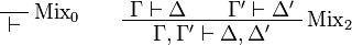
| + | === Mix rules === |
||
| + | |||
| + | It is quite common to consider [[Mix|mix rules]]: |
||
<math> |
<math> |
||
| − | \AxRule{ \Gamma, A \vdash \Delta } |
+ | \LabelRule{\rulename{Mix}_0} |
| − | \LabelRule{ d } |
+ | \NulRule{\vdash} |
| − | \UnaRule{ \Gamma, \oc A \vdash \Delta } |
||
\DisplayProof |
\DisplayProof |
||
\qquad |
\qquad |
||
| − | \AxRule{ \Gamma \vdash \Delta } |
+ | \AxRule{\Gamma \vdash \Delta} |
| − | \LabelRule{ w } |
+ | \AxRule{\Gamma' \vdash \Delta'} |
| − | \UnaRule{ \Gamma, \oc A \vdash \Delta } |
+ | \LabelRule{\rulename{Mix}_2} |
| − | \DisplayProof |
+ | \BinRule{\Gamma,\Gamma' \vdash \Delta,\Delta'} |
| − | \qquad |
||
| − | \AxRule{ \Gamma, \oc A, \oc A \vdash \Delta } |
||
| − | \LabelRule{ c } |
||
| − | \UnaRule{ \Gamma, \oc A \vdash \Delta } |
||
| − | \DisplayProof |
||
| − | \qquad |
||
| − | \AxRule{ \oc A_1, \ldots, \oc A_n \vdash B } |
||
| − | \LabelRule{ \oc_R } |
||
| − | \UnaRule{ \oc A_1, \ldots, \oc A_n \vdash \oc B } |
||
\DisplayProof |
\DisplayProof |
||
</math> |
</math> |
||
Latest revision as of 16:46, 28 October 2013
This article presents the language and sequent calculus of second-order linear logic and the basic properties of this sequent calculus. The core of the article uses the two-sided system with negation as a proper connective; the one-sided system, often used as the definition of linear logic, is presented at the end of the page.
Contents |
[edit] Formulas
Atomic formulas, written α,β,γ, are predicates of
the form  , where the ti are terms
from some first-order language.
The predicate symbol p may be either a predicate constant or a
second-order variable.
By convention we will write first-order variables as x,y,z,
second-order variables as X,Y,Z, and ξ for a
variable of arbitrary order (see Notations).
, where the ti are terms
from some first-order language.
The predicate symbol p may be either a predicate constant or a
second-order variable.
By convention we will write first-order variables as x,y,z,
second-order variables as X,Y,Z, and ξ for a
variable of arbitrary order (see Notations).
Formulas, represented by capital letters A, B, C, are built using the following connectives:
| α | atom | 
|
negation | |

|
tensor | 
|
par | multiplicatives |

|
one | 
|
bottom | multiplicative units |

|
plus | 
|
with | additives |

|
zero | 
|
top | additive units |

|
of course | 
|
why not | exponentials |

|
there exists | 
|
for all | quantifiers |
Each line (except the first one) corresponds to a particular class of
connectives, and each class consists in a pair of connectives.
Those in the left column are called positive and those in
the right column are called negative.
The tensor and with connectives are conjunctions while par and
plus are disjunctions.
The exponential connectives are called modalities, and traditionally read
of course A for and why not
A for .
Quantifiers may apply to first- or second-order variables.
There is no connective for implication in the syntax of standard linear logic.
Instead, a linear implication is defined similarly to the decomposition
 in classical logic, as
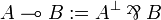 .
.
Free and bound variables and first-order substitution are defined in the
standard way.
Formulas are always considered up to renaming of bound names.
If A is a formula, X is a second-order variable and
![B[x_1,\ldots,x_n]](/mediawiki/images/math/3/a/d/3ad43a5c556e19246b33673d45dd904d.png) is a formula with variables xi,
then the formula A[B / X] is A where every atom
is a formula with variables xi,
then the formula A[B / X] is A where every atom
 is replaced by
 ![B[t_1,\ldots,t_n]](/mediawiki/images/math/6/e/4/6e405b754714c3b72973cc1fe9b9ec42.png) .
.
[edit] Sequents and proofs
A sequent is an expression  where
Γ and Δ are finite multisets of formulas.
For a multiset
where
Γ and Δ are finite multisets of formulas.
For a multiset  , the notation
 represents the multiset
 .
Proofs are labelled trees of sequents, built using the following inference
rules:
.
Proofs are labelled trees of sequents, built using the following inference
rules:
- Identity group:
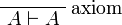
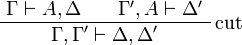
- Negation:
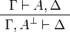
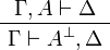
- Multiplicative group:
- tensor:
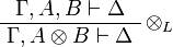
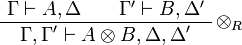
- par:
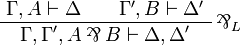
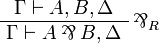
- one:
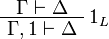

- bottom:

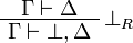
- tensor:
- Additive group:
- plus:
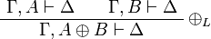
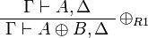
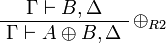
- with:
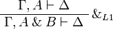
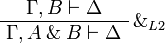
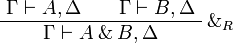
- zero:
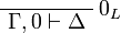
- top:
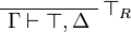
- plus:
- Exponential group:
- of course:
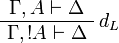
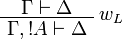
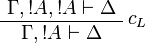
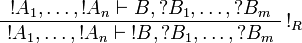
- why not:
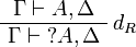
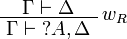
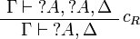
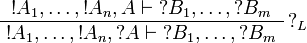
- of course:
- Quantifier group (in the
 and
and  rules, ξ must not occur free in Γ or Δ):
- there exists:
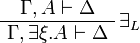
![\AxRule{ \Gamma \vdash \Delta, A[t/x] }
\LabelRule{ \exists^1_R }
\UnaRule{ \Gamma \vdash \Delta, \exists x.A }
\DisplayProof](/mediawiki/images/math/3/3/c/33cd98d69ac858f40d7a231d96037aea.png)
![\AxRule{ \Gamma \vdash \Delta, A[B/X] }
\LabelRule{ \exists^2_R }
\UnaRule{ \Gamma \vdash \Delta, \exists X.A }
\DisplayProof](/mediawiki/images/math/9/6/b/96b94853d6eac425879ceef1583f5e84.png)
- for all:
![\AxRule{ \Gamma, A[t/x] \vdash \Delta }
\LabelRule{ \forall^1_L }
\UnaRule{ \Gamma, \forall x.A \vdash \Delta }
\DisplayProof](/mediawiki/images/math/1/a/3/1a33210d9d315018d6489ce6bab92ea7.png)
![\AxRule{ \Gamma, A[B/X] \vdash \Delta }
\LabelRule{ \forall^2_L }
\UnaRule{ \Gamma, \forall X.A \vdash \Delta }
\DisplayProof](/mediawiki/images/math/7/6/8/768bcb3e8ddcd5c483cd40839b4a035c.png)
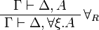
- there exists:
The left rules for of course and right rules for why not are called
dereliction, weakening and contraction rules.
The right rule for of course and the left rule for why not are called
promotion rules.
Note the fundamental fact that there are no contraction and weakening rules
for arbitrary formulas, but only for the formulas starting with the
 modality.
This is what distinguishes linear logic from classical logic: if weakening and
contraction were allowed for arbitrary formulas, then
modality.
This is what distinguishes linear logic from classical logic: if weakening and
contraction were allowed for arbitrary formulas, then  and
and  would be identified, as well as
  and
and  , and ,
and .
By identified, we mean here that replacing a with a or
vice versa would preserve provability.
, and ,
and .
By identified, we mean here that replacing a with a or
vice versa would preserve provability.
Sequents are considered as multisets, in other words as sequences up to permutation. An alternative presentation would be to define a sequent as a finite sequence of formulas and to add the exchange rules:
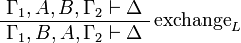
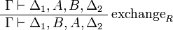
[edit] Equivalences
Two formulas A and B are (linearly) equivalent,
written  , if both implications
  and
and  are provable.
Equivalently, if both
are provable.
Equivalently, if both  and
and
 are provable.
Another formulation of is that, for all
Γ and Δ,
are provable.
Another formulation of is that, for all
Γ and Δ,  is provable if and only if
  is provable.
Two related notions are isomorphism (stronger than equivalence) and equiprovability (weaker than equivalence).
[edit] De Morgan laws
Negation is involutive:

Duality between connectives:

|
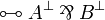
|

|
| |

|

|

|

| |

|
|

|
| |

|

|

|

| |

|

|

|

| |

|

|

|

|
[edit] Fundamental equivalences
- Associativity, commutativity, neutrality:
-
- Idempotence of additives:
-
- Distributivity of multiplicatives over additives:
-
- Defining property of exponentials:
-
- Monoidal structure of exponentials:
-
- Digging:
-
- Other properties of exponentials:
-


These properties of exponentials lead to the lattice of exponential modalities.
- Commutation of quantifiers (ζ does not occur in A):
-
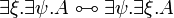


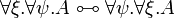

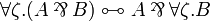

[edit] Definability
The units and the additive connectives can be defined using second-order quantification and exponentials, indeed the following equivalences hold:

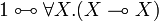

The constants and and the connective
can be defined by duality.
Any pair of connectives that has the same rules as  is
equivalent to it, the same holds for additives, but not for exponentials.
is
equivalent to it, the same holds for additives, but not for exponentials.
Other basic equivalences exist.
[edit] Properties of proofs
[edit] Cut elimination and consequences
Theorem (cut elimination)
For every sequent , there is a proof of
if and only if there is a proof of
that does not use the cut rule.
This property is proved using a set of rewriting rules on proofs, using appropriate termination arguments (see the specific articles on cut elimination for detailed proofs), it is the core of the proof/program correspondence.
It has several important consequences:
Definition (subformula)
The subformulas of a formula A are A and, inductively, the subformulas of its immediate subformulas:
- the immediate subformulas of , , , are A and B,
- the only immediate subformula of and is A,
- , , , and atomic formulas have no immediate subformula,
- the immediate subformulas of
 and
and  are all the A[t / x] for all first-order terms t,
- the immediate subformulas of
 and
and  are all the A[B / X] for all formulas B (with the appropriate number of parameters).
Theorem (subformula property)
A sequent is provable if and only if it is the conclusion of a proof in which each intermediate conclusion is made of subformulas of the
formulas of Γ and Δ.
Proof. By the cut elimination theorem, if a sequent is provable, then it is provable by a cut-free proof. In each rule except the cut rule, all formulas of the premisses are either formulas of the conclusion, or immediate subformulas of it, therefore cut-free proofs have the subformula property.
The subformula property means essentially nothing in the second-order system, since any formula is a subformula of a quantified formula where the quantified variable occurs. However, the property is very meaningful if the sequent Γ does not use second-order quantification, as it puts a strong restriction on the set of potential proofs of a given sequent. In particular, it implies that the first-order fragment without quantifiers is decidable.
Theorem (consistency)
The empty sequent  is not provable.
Subsequently, it is impossible to prove both a formula A and its
negation ; it is impossible to prove or
.
is not provable.
Subsequently, it is impossible to prove both a formula A and its
negation ; it is impossible to prove or
.
Proof. If a sequent is provable, then it is the conclusion of a cut-free proof.
In each rule except the cut rule, there is at least one formula in conclusion.
Therefore cannot be the conclusion of a proof.
The other properties are immediate consequences: if  and
and  are provable, then by the left negation rule
 is provable, and by the cut rule one gets empty
conclusion, which is not possible.
As particular cases, since and are
provable, and are not, since they are
equivalent to and
respectively.
is provable, and by the cut rule one gets empty
conclusion, which is not possible.
As particular cases, since and are
provable, and are not, since they are
equivalent to and
respectively.
[edit] Expansion of identities
Let us write  to signify that
π is a proof with conclusion .
to signify that
π is a proof with conclusion .
Proposition (η-expansion)
For every proof π, there is a proof π' with the
same conclusion as π in which the axiom rule is only used with
atomic formulas.
If π is cut-free, then there is a cut-free π'.
Proof. It suffices to prove that for every formula A, the sequent
 has a cut-free proof in which the axiom rule is used
only for atomic formulas.
We prove this by induction on A.
has a cut-free proof in which the axiom rule is used
only for atomic formulas.
We prove this by induction on A.
- If A is atomic, then is an instance of the atomic axiom rule.
- If
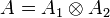 then we have
where π1 and π2 exist by induction hypothesis. - If
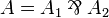 then we have
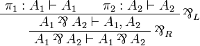
where π1 and π2 exist by induction hypothesis. - All other connectives follow the same pattern.
The interesting thing with η-expansion is that, we can always assume that
each connective is explicitly introduced by its associated rule (except in the
case where there is an occurrence of the rule).
[edit] Reversibility
Definition (reversibility)
A connective c is called reversible if
- for every proof
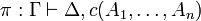 , there is a proof π' with the same conclusion in which
 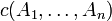 is introduced by the last rule,
- if π is cut-free then there is a cut-free π'.
Proposition
The connectives , , , and  are reversible.
Proof. Using the η-expansion property, we assume that the axiom rule is only applied to atomic formulas.
Then each top-level connective is introduced either by its associated (left or
right) rule or in an instance of the  or
or
 rule.
rule.
For , consider a proof 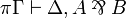 .
If is introduced by a
.
If is introduced by a  rule (not
necessarily the last rule in π), then if we remove this rule
we get a proof of
rule (not
necessarily the last rule in π), then if we remove this rule
we get a proof of  (this can be proved by a
straightforward induction on π).
If it is introduced in the context of a or
rule, then this rule can be changed so that
is replaced by A,B.
In either case, we can apply a final rule to get the
expected proof.
(this can be proved by a
straightforward induction on π).
If it is introduced in the context of a or
rule, then this rule can be changed so that
is replaced by A,B.
In either case, we can apply a final rule to get the
expected proof.
For , the same technique applies: if it is introduced by a
 rule, then remove this rule to get a proof of
 , if it is introduced by a or
rule, remove the from this rule, then
apply the rule at the end of the new proof.
, if it is introduced by a or
rule, remove the from this rule, then
apply the rule at the end of the new proof.
For , consider a proof
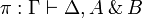 .
If the connective is introduced by a rule then this rule is
applied in a context like
.
If the connective is introduced by a rule then this rule is
applied in a context like
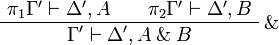
Since the formula is not involved in other rules (except
as context), if we replace this step by π1 in π
we finally get a proof 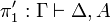 .
If we replace this step by π2 we get a proof
.
If we replace this step by π2 we get a proof
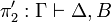 .
Combining π1 and π2 with a final
rule we finally get the expected proof.
The case when the was introduced in a
rule is solved as before.
.
Combining π1 and π2 with a final
rule we finally get the expected proof.
The case when the was introduced in a
rule is solved as before.
For the result is trivial: just choose π' as
an instance of the rule with the appropriate conclusion.
For , consider a proof
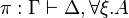 .
Up to renaming, we can assume that ξ occurs free only above the
rule that introduces the quantifier.
If the quantifier is introduced by a rule, then if we
remove this rule, we can check that we get a proof of
on which we can finally apply the
rule.
The case when the was introduced in a
rule is solved as before.
.
Up to renaming, we can assume that ξ occurs free only above the
rule that introduces the quantifier.
If the quantifier is introduced by a rule, then if we
remove this rule, we can check that we get a proof of
on which we can finally apply the
rule.
The case when the was introduced in a
rule is solved as before.
Note that, in each case, if the proof we start from is cut-free, our
transformations do not introduce a cut rule.
However, if the original proof has cuts, then the final proof may have more
cuts, since in the case of we duplicated a part of the
original proof.
A corresponding property for positive connectives is focalization, which states that clusters of positive formulas can be treated in one step, under certain circumstances.
[edit] One-sided sequent calculus
The sequent calculus presented above is very symmetric: for every left
introduction rule, there is a right introduction rule for the dual connective
that has the exact same structure.
Moreover, because of the involutivity of negation, a sequent
 is provable if and only if the sequent
 is provable.
From these remarks, we can define an equivalent one-sided sequent calculus:
is provable.
From these remarks, we can define an equivalent one-sided sequent calculus:
- Formulas are considered up to De Morgan duality. Equivalently, one can consider that negation is not a connective but a syntactically defined operation on formulas. In this case, negated atoms
 must be considered as another kind of atomic formulas.
- Sequents have the form .
The inference rules are essentially the same except that the left hand side of sequents is kept empty:
- Identity group:
-
- Multiplicative group:
-
- Additive group:
-
- Exponential group:
-
- Quantifier group (in the rule, ξ must not occur free in Γ):
-
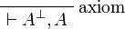
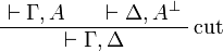
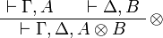
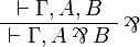


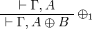
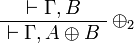
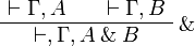


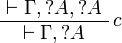

![\AxRule{ \vdash \Gamma, A[t/x] }
\LabelRule{ \exists^1 }
\UnaRule{ \vdash \Gamma, \exists x.A }
\DisplayProof](/mediawiki/images/math/2/b/6/2b689e6be9aae26140ef3056c37f576b.png)
![\AxRule{ \vdash \Gamma, A[B/X] }
\LabelRule{ \exists^2 }
\UnaRule{ \vdash \Gamma, \exists X.A }
\DisplayProof](/mediawiki/images/math/9/f/1/9f1d81fcdbb7913777097d7577cf0f1e.png)
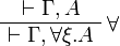
Theorem
A two-sided sequent is provable if
and only if the sequent  is provable in
the one-sided system.
is provable in
the one-sided system.
The one-sided system enjoys the same properties as the two-sided one, including cut elimination, the subformula property, etc. This formulation is often used when studying proofs because it is much lighter than the two-sided form while keeping the same expressiveness. In particular, proof-nets can be seen as a quotient of one-sided sequent calculus proofs under commutation of rules.
[edit] Variations
[edit] Exponential rules
- The promotion rule, on the right-hand side for example,
can be replaced by a multi-functorial promotion rule
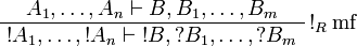 and a digging rule
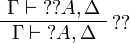 ,
without modifying the provability.
,
without modifying the provability.
Note that digging violates the subformula property.
- In presence of the digging rule , the multiplexing rule
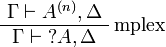 (where A(n) stands for n occurrences of formula A) is equivalent (for provability) to the triple of rules: contraction, weakening, dereliction.
[edit] Non-symmetric sequents
The same remarks that lead to the definition of the one-sided calculus can lead the definition of other simplified systems:
- A one-sided variant with sequents of the form
 could be defined.
- When considering formulas up to De Morgan duality, an equivalent system is obtained by considering only the left and right rules for positive connectives (or the ones for negative connectives only, obviously).
- Intuitionistic linear logic is the two-sided system where the right-hand side is constrained to always contain exactly one formula (with a few associated restrictions).
- Similar restrictions are used in various semantics and proof search formalisms.
[edit] Mix rules
It is quite common to consider mix rules: