Finiteness semantics

Revision as of 23:43, 25 May 2009

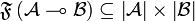
The category $\mathbf{Fin}$ of finiteness spaces and finitary relations was introduced by Ehrhard, refining the purely relational model of linear logic. A finiteness space is a set equipped with a finiteness structure, i.e. a particular set of subsets which are said to be finitary; and the model is such that the usual relational denotation of a proof in linear logic is always a finitary subset of its conclusion. By the usual co-Kleisli construction, this also provides a model of the simply typed lambda-calculus: the cartesian closed category $\mathbf{Fin}_\oc$ .

The main property of finiteness spaces is that the intersection of two finitary subsets of dual types is always finite. This feature allows to reformulate Girard's quantitative semantics in a standard algebraic setting, where morphisms interpreting typed $λ$ -terms are analytic functions between the topological vector spaces generated by vectors with finitary supports. This provided the semantical foundations of Ehrhard-Regnier's differential $λ$ -calculus and motivated the general study of a differential extension of linear logic.

It is worth noticing that finiteness spaces can accomodate typed $λ$ -calculi only: for instance, the relational semantics of fixpoint combinators is never finitary. The whole point of the finiteness construction is actually to reject infinite computations. Indeed, from a logical point of view, computation is cut elimination: the finiteness structure ensures the intermediate sets involved in the relational interpretation of a cut are all finite. In that sense, the finitary semantics is intrinsically typed.

Finiteness spaces

The construction of finiteness spaces follows a well known pattern. It is given by the following notion of orthogonality: $a\mathrel \bot a'$ iff $a\cap a'$ is finite. Then one unrolls familiar definitions, as we do in the following paragraphs.

Let $A$ be a set. Denote by $\mathfrak P(A)$ the powerset of $A$ and by $\mathfrak P_f(A)$ the set of all finite subsets of $A$ . Let ${\mathfrak F} \subseteq \mathfrak P(A)$ any set of subsets of $A$ . We define the pre-dual of ${\mathfrak F}$ in $A$ as ${\mathfrak F}^{\bot_{A}}=\left\{a'\subseteq A;\ \forall a\in{\mathfrak F},\ a\cap a'\in\mathfrak P_f(A)\right\}$ . In general we will omit the subscript in the pre-dual notation and just write ${\mathfrak F}\orth$ . For all ${\mathfrak F}\subseteq\mathfrak P(A)$ , we have the following immediate properties: $\mathfrak P_f(A) \subseteq {\mathfrak F}\orth$ ; ${\mathfrak F}\subseteq {\mathfrak F}\biorth$ ; if ${\mathfrak G}\subseteq{\mathfrak F}$ , ${\mathfrak F}\orth\subseteq {\mathfrak G}\orth$ . By the last two, we get ${\mathfrak F}\orth = {\mathfrak F}\triorth$ . A finiteness structure on $A$ is then a set ${\mathfrak F}$ of subsets of $A$ such that ${\mathfrak F}\biorth = {\mathfrak F}$ .

A finiteness space is a dependant pair ${\mathcal A}=\left(\web{\mathcal A},\mathfrak F\left(\mathcal A\right)\right)$ where $\web {\mathcal A}$ is the underlying set (the web of ${\mathcal A}$ ) and $\mathfrak F\left(\mathcal A\right)$ is a finiteness structure on $\web {\mathcal A}$ . We then write ${\mathcal A}\orth$ for the dual finiteness space: $\web {{\mathcal A}\orth} = \web {\mathcal A}$ and $\mathfrak F\left({\mathcal A}\orth\right)=\mathfrak F\left({\mathcal A}\right)^{\bot}$ . The elements of $\mathfrak F\left(\mathcal A\right)$ are called the finitary subsets of ${\mathcal A}$ .

Example.

For all set $A$ , $(A,\mathfrak P_f(A))$ is a finiteness space and $(A,\mathfrak P_f(A))\orth = (A,\mathfrak P(A))$ . In particular, each finite set $A$ is the web of exactly one finiteness space: $(A,\mathfrak P_f(A))=(A,\mathfrak P(A))$ . We introduce the following two: $\zero = \zero\orth = \left(\emptyset, \{\emptyset\}\right)$ and $\one = \one\orth = \left(\{\emptyset\}, \{\emptyset, \{\emptyset\}\}\right)$ . We also introduce the finiteness space of natural numbers ${\mathcal N}$ by: $|{\mathcal N}|={\mathbf N}$ and $a\in\mathfrak F\left(\mathcal N\right)$ iff $a$ is finite. We write $\mathcal O=\{0\}\in\mathfrak F\left({\mathcal N}\right)$ .

Notice that ${\mathfrak F}$ is a finiteness structure iff it is of the form ${\mathfrak G}\orth$ . It follows that any finiteness structure ${\mathfrak F}$ is downwards closed for inclusion, and closed under finite unions and arbitrary intersections. Notice however that ${\mathfrak F}$ is not closed under directed unions in general: for all $k\in{\mathbf N}$ , write $k{\downarrow}=\left\{j;\ j\le k\right\}\in\mathfrak F\left({\mathcal N}\right)$ ; then $k{\downarrow}\subseteq k'{\downarrow}$ as soon as $k\le k'$ , but $\bigcup_{k\ge0} k{\downarrow}={\mathbf N}\not\in\mathfrak F\left({\mathcal N}\right)$ .

Multiplicatives

For all finiteness spaces ${\mathcal A}$ and ${\mathcal B}$ , we define ${\mathcal A} \tens {\mathcal B}$ by $\web {{\mathcal A} \tens {\mathcal B}} = \web{\mathcal A} \times \web{\mathcal B}$ and $\mathfrak F\left({\mathcal A} \tens {\mathcal B}\right) = \left\{a\times b;\ a\in \mathfrak F\left(\mathcal A\right),\ b\in\mathfrak F\left(\mathcal B\right)\right\}\biorth$ . It can be shown that $\mathfrak F\left({\mathcal A} \tens {\mathcal B}\right) = \left\{ c \subseteq \web{\mathcal A}\times\web{\mathcal B};\ \left.c\right|_l\in \mathfrak F\left(\mathcal A\right),\ \left.c\right|_r\in\mathfrak F\left(\mathcal B\right)\right\}$ , where $\left.c\right|_l$ and $\left.c\right|_r$ are the obvious projections.

Let $f\subseteq A \times B$ be a relation from $A$ to $B$ , we write $f\orth=\left\{(\beta,\alpha);\ (\alpha,\beta)\in f\right\}$ . For all $a\subseteq A$ , we set $f\cdot a = \left\{\beta\in B;\ \exists \alpha\in a,\ (\alpha,\beta)\in f\right\}$ . If moreover $g\subseteq B \times C$ , we define $g \bullet f = \left\{(\alpha,\gamma)\in A\times C;\ \exists \beta\in B,\ (\alpha,\beta)\in f\wedge(\beta,\gamma)\in g\right\}$ . Then, setting ${\mathcal A}\limp{\mathcal B} = \left({\mathcal A}\otimes {\mathcal B}\orth\right)\orth$ , $\mathfrak F\left({\mathcal A}\limp{\mathcal B}\right)\subseteq {\web{\mathcal A}\times\web{\mathcal B}}$ is characterized as follows:

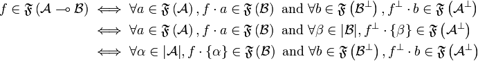
$\begin{align} f\in \mathfrak F\left({\mathcal A}\limp{\mathcal B}\right) &\iff \forall a\in \mathfrak F\left({\mathcal A}\right), f\cdot a \in\mathfrak F\left({\mathcal B}\right) \text{ and } \forall b\in \mathfrak F\left({\mathcal B}\orth\right), f\orth\cdot b \in\mathfrak F\left({\mathcal A}\orth\right) \\ &\iff \forall a\in \mathfrak F\left({\mathcal A}\right), f\cdot a \in\mathfrak F\left({\mathcal B}\right) \text{ and } \forall \beta\in \web{{\mathcal B}}, f\orth\cdot \left\{\beta\right\} \in\mathfrak F\left({\mathcal A}\orth\right) \\ &\iff \forall \alpha\in \web{{\mathcal A}}, f\cdot \left\{\alpha\right\} \in\mathfrak F\left({\mathcal B}\right) \text{ and } \forall b\in \mathfrak F\left({\mathcal B}\orth\right), f\orth\cdot b \in\mathfrak F\left({\mathcal A}\orth\right) \end{align}$

The elements of $\mathfrak F\left({\mathcal A}\limp{\mathcal B}\right)$ are called finitary relations from ${\mathcal A}$ to ${\mathcal B}$ . By the previous characterization, the identity relation 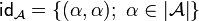$\mathsf{id}_{{\mathcal A}} = \left\{(\alpha,\alpha);\ \alpha\in\web{{\mathcal A}}\right\}$ is finitary, and the composition of two finitary relations is also finitary. One can thus define the category $\mathbf{Fin}$ of finiteness spaces and finitary relations: the objects of $\mathbf{Fin}$ are all finiteness spaces, and 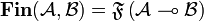$\mathbf{Fin}({\mathcal A},{\mathcal B})=\mathfrak F\left({\mathcal A}\limp{\mathcal B}\right)$ . Equipped with the tensor product $\tens$ , $\mathbf{Fin}$ is symmetric monoidal, with unit $\one$ ; it is monoidal closed by the definition of $\limp$ ; it is $*$ -autonomous by the obvious isomorphism between ${\mathcal A}\orth$ and ${\mathcal A}\limp\one$ .

Example.

Setting $\mathcal{S}=\left\{(k,k+1);\ k\in{\mathbf N}\right\}$ and $\mathcal{P}=\left\{(k+1,k);\ k\in{\mathbf N}\right\}$ , we have $\mathcal{S},\mathcal{P}\in\mathbf{Fin}({\mathcal N},{\mathcal N})$ and $\mathcal{P}\bullet\mathcal{S}=\mathsf{id}_{{\mathcal N}}$ .

Additives

We now introduce the cartesian structure of $\mathbf{Fin}$ . We define ${\mathcal A} \oplus {\mathcal B}$ by $\web {{\mathcal A} \oplus {\mathcal B}} = \web{\mathcal A} \uplus \web{\mathcal B}$ and $\mathfrak F\left({\mathcal A} \oplus {\mathcal B}\right) = \left\{ a\uplus b;\ a\in \mathfrak F\left(\mathcal A\right),\ b\in\mathfrak F\left(\mathcal B\right)\right\}$ where $\uplus$ denotes the disjoint union of sets: $x\uplus y=(\{1\}\times x)\cup(\{2\}\times y)$ . We have $\left({\mathcal A}\oplus {\mathcal B}\right)\orth = {\mathcal A}\orth\oplus{\mathcal B}\orth$ . The category $\mathbf{Fin}$ is both cartesian and co-cartesian, with $\oplus$ being the product and co-product, and $\zero$ the initial and terminal object. Projections are given by: \begin{eqnarray*} \lambda_{{\mathcal A},{\mathcal B}}&=&\left\{\left((1,\alpha),\alpha\right);\ \alpha\in\web{\mathcal A}\right\} \in\mathbf{Fin}({\mathcal A}\oplus{\mathcal B},{\mathcal A}) \\ \rho_{{\mathcal A},{\mathcal B}}&=&\left\{\left((2,\beta),\beta\right);\ \beta\in\web{\mathcal B}\right\} \in\mathbf{Fin}({\mathcal A}\oplus{\mathcal B},{\mathcal B}) \end{eqnarray*} and if $f\in\mathbf{Fin}({\mathcal C},{\mathcal A})$ and $g\in\mathbf{Fin}({\mathcal C},{\mathcal B})$ , pairing is given by:

$\left\langle f,g\right\rangle = \left\{\left(\gamma,(1,\alpha)\right);\ (\gamma,\alpha)\in f\right\} \cup \left\{\left(\gamma,(2,\beta)\right);\ (\gamma,\beta)\in g\right\} \in\mathbf{Fin}({\mathcal C},{\mathcal A}\oplus{\mathcal B}).$

The unique morphism from ${\mathcal A}$ to $\zero$ is the empty relation. The co-cartesian structure is obtained symmetrically.

Example.

Write ${\mathcal O}\orth=\left\{(0,\emptyset)\right\}\in\mathbf{Fin}({\mathcal N},\one)$ . Then $\left\langle{{\mathcal O}\orth},{\mathcal{P}}\right\rangle =\{ (0,(1,\emptyset)) \}\cup \{ (k+1,(2,k)) ;\ k\in{\mathbf N} \} \in\mathbf{Fin}\left({\mathcal N},\one\oplus{\mathcal N}\right)$ is an isomorphism.

Exponentials

If $A$ is a set, we denote by $\mathfrak M_f(A)$ the set of all finite multisets of elements of $A$ , and if $a\subseteq A$ , we write $a^{\oc}=\mathfrak M_f(a)\subseteq\mathfrak M_f(A)$ . If $\overline\alpha\in\mathfrak M_f(A)$ , we denote its support by $\mathrm{Support}\left(\overline \alpha\right)\in\mathfrak P_f(A)$ . For all finiteness space ${\mathcal A}$ , we define $\oc {\mathcal A}$ by: $\web{\oc {\mathcal A}}= \mathfrak M_f\left(\web{{\mathcal A}}\right)$ and $\mathfrak F\left(\oc{\mathcal A}\right)=\left\{a^{\oc};\ a\in\mathfrak F\left({\mathcal A}\right)\right\}\biorth$ . 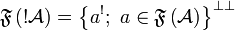It can be shown that $\mathfrak F\left(\oc{\mathcal A}\right) = \left\{\overline a\subseteq\mathfrak M_f\left(\web{{\mathcal A}}\right);\ \bigcup_{\overline\alpha\in \overline a}\mathrm{Support}\left(\overline \alpha\right)\in\mathfrak F\left(\mathcal A\right)\right\}$ . 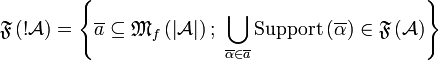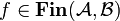Then, for all $f\in\mathbf{Fin}({\mathcal A},{\mathcal B})$ , we set

$\oc f =\left\{\left(\left[\alpha_1,\ldots,\alpha_n\right],\left[\beta_1,\ldots,\beta_n\right]\right);\ \forall i,\ (\alpha_i,\beta_i)\in f\right\} \in \mathbf{Fin}(\oc {\mathcal A}, \oc {\mathcal B}),$

which defines a functor. Natural transformations $\mathsf{der}_{{\mathcal A}}=\left\{([\alpha],\alpha);\ \alpha\in \web{{\mathcal A}}\right\}\in\mathbf{Fin}(\oc{\mathcal A},{\mathcal A})$ and $\mathsf{digg}_{{\mathcal A}}=\left\{\left(\sum_{i=1}^n\overline\alpha_i,\left[\overline\alpha_1,\ldots,\overline\alpha_n\right]\right);\ \forall i,\ \overline\alpha_i\in\web{\oc {\mathcal A}}\right\}$ make this functor a comonad.

Example.

We have isomorphisms $\left\{([],\emptyset)\right\}\in\mathbf{Fin}(\oc\zero,\one)$ and

$\left\{ \left(\overline\alpha_l+\overline\beta_r,\left(\overline\alpha,\overline\beta\right)\right);\ (\overline\alpha_l,\overline\alpha)\in\oc\lambda_{{\mathcal A},{\mathcal B}}\wedge(\overline\beta_r,\overline\beta)\in\oc\rho_{{\mathcal A},{\mathcal B}}\right\} \in\mathbf{Fin}(\oc({\mathcal A}\oplus{\mathcal B}),\oc{\mathcal A}\tens\oc{\mathcal B}).$

More generally, we have $\oc\left({\mathcal A}_1\oplus\cdots\oplus{\mathcal A}_n\right)\cong\oc{\mathcal A}_1\tens\cdots\tens\oc{\mathcal A}_n$ .

@@ Line 23: / Line 23: @@
 Let <math>f\subseteq A \times B</math> be a relation from <math>A</math> to <math>B</math>, we write <math>f\orth=\left\{(\beta,\alpha);\  (\alpha,\beta)\in f\right\}</math>.  For all <math>a\subseteq A</math>, we set <math>f\cdot a = \left\{\beta\in B;\  \exists \alpha\in a,\ (\alpha,\beta)\in f\right\}</math>.  If moreover <math>g\subseteq B \times C</math>, we define <math>g \bullet f = \left\{(\alpha,\gamma)\in A\times C;\  \exists \beta\in B,\ (\alpha,\beta)\in f\wedge(\beta,\gamma)\in g\right\}</math>.  Then, setting <math>{\mathcal A}\limp{\mathcal B} = \left({\mathcal A}\otimes {\mathcal B}\orth\right)\orth</math>, <math>\mathfrak F\left({\mathcal A}\limp{\mathcal B}\right)\subseteq {\web{\mathcal A}\times\web{\mathcal B}}</math> is characterized as follows:
-\begin{center}
-	\begin{tabular}{r@{\ iff\ }l}
+<math>
-		<math>f\in \mathfrak F\left({\mathcal A}\limp{\mathcal B}\right)</math> & <math>\forall a\in \mathfrak F\left({\mathcal A}\right)</math>, <math>f\cdot a \in\mathfrak F\left({\mathcal B}\right)</math> and <math>\forall b\in \mathfrak F\left({\mathcal B}\orth\right)</math>, <math>f\orth\cdot b \in\mathfrak F\left({\mathcal A}\orth\right)</math>
+\begin{align}
+		f\in \mathfrak F\left({\mathcal A}\limp{\mathcal B}\right) &\iff \forall a\in \mathfrak F\left({\mathcal A}\right), f\cdot a \in\mathfrak F\left({\mathcal B}\right) \text{ and } \forall b\in \mathfrak F\left({\mathcal B}\orth\right), f\orth\cdot b \in\mathfrak F\left({\mathcal A}\orth\right)
 		\\
-		& <math>\forall a\in \mathfrak F\left({\mathcal A}\right)</math>, <math>f\cdot a \in\mathfrak F\left({\mathcal B}\right)</math> and <math>\forall \beta\in \web{{\mathcal B}}</math>, <math>f\orth\cdot \left\{\beta\right\} \in\mathfrak F\left({\mathcal A}\orth\right)</math>
+		&\iff \forall a\in \mathfrak F\left({\mathcal A}\right), f\cdot a \in\mathfrak F\left({\mathcal B}\right) \text{ and } \forall \beta\in \web{{\mathcal B}}, f\orth\cdot \left\{\beta\right\} \in\mathfrak F\left({\mathcal A}\orth\right)
 		\\
-		& <math>\forall \alpha\in \web{{\mathcal A}}</math>, <math>f\cdot \left\{\alpha\right\} \in\mathfrak F\left({\mathcal B}\right)</math> and <math>\forall b\in \mathfrak F\left({\mathcal B}\orth\right)</math>, <math>f\orth\cdot b \in\mathfrak F\left({\mathcal A}\orth\right)</math>
+		&\iff \forall \alpha\in \web{{\mathcal A}}, f\cdot \left\{\alpha\right\} \in\mathfrak F\left({\mathcal B}\right) \text{ and } \forall b\in \mathfrak F\left({\mathcal B}\orth\right), f\orth\cdot b \in\mathfrak F\left({\mathcal A}\orth\right)
-	\end{tabular}
+\end{align}
-\end{center}
+</math>
 The elements of <math>\mathfrak F\left({\mathcal A}\limp{\mathcal B}\right)</math> are called finitary relations from <math>{\mathcal A}</math> to <math>{\mathcal B}</math>. By the previous characterization, the identity relation <math>\mathsf{id}_{{\mathcal A}} = \left\{(\alpha,\alpha);\  \alpha\in\web{{\mathcal A}}\right\}</math> is finitary, and the composition of two finitary relations is also finitary. One can thus define the category <math>\mathbf{Fin}</math> of finiteness spaces and finitary relations: the objects of <math>\mathbf{Fin}</math> are all finiteness spaces, and <math>\mathbf{Fin}({\mathcal A},{\mathcal B})=\mathfrak F\left({\mathcal A}\limp{\mathcal B}\right)</math>.  Equipped with the tensor product <math>\tens</math>, <math>\mathbf{Fin}</math> is symmetric monoidal, with unit <math>\one</math>; it is monoidal closed by the definition of <math>\limp</math>; it is <math>*</math>-autonomous by the obvious isomorphism between <math>{\mathcal A}\orth</math> and <math>{\mathcal A}\limp\one</math>.
 <!--  By contrast with the purely relational model, it is not compact closed:  -->
@@ Line 39: / Line 39: @@
 ===== Example. =====
 	Setting <math>\mathcal{S}=\left\{(k,k+1);\  k\in{\mathbf N}\right\}</math> and <math>\mathcal{P}=\left\{(k+1,k);\  k\in{\mathbf N}\right\}</math>, we have <math>\mathcal{S},\mathcal{P}\in\mathbf{Fin}({\mathcal N},{\mathcal N})</math> and <math>\mathcal{P}\bullet\mathcal{S}=\mathsf{id}_{{\mathcal N}}</math>.
 === Additives ===

Finiteness semantics

Revision as of 23:43, 25 May 2009

Contents

Finiteness spaces

Example.

Multiplicatives

Example.

Additives

Example.

Exponentials

Example.

Views

Personal tools

Navigation

Search

Tools